After more than a century of polar exploration, recent satellite measurements are painting an altogether new picture of Antarctica. Andrew Shepherd explains how physics is helping researchers understand the critical transformations taking place in the world's largest ice sheet

Antarctica is the world’s last great wilderness. Desolate, cold and largely unspoilt by humans, the continent provides a natural habitat for penguins, seals, whales and other wildlife. It is also home to the largest reservoir of fresh water anywhere on Earth, in the form of a vast sheet of ice that covers almost all of its land. Bounded by icy peaks, dry valleys and the southern oceans, this sheet plays a key role in the Earth’s hydrological cycle.
Every year a volume of water equivalent to the upper 7 mm of all of our planet’s oceans falls as snow on the Antarctic ice sheet, while a roughly equivalent amount of ice slips into the sea via glaciers. But the ice sheet is seldom in a state of balance. From one ice age to the next, and from one season to the next, the amount of snow arriving differs from the amount of ice leaving, causing parts of Antarctica’s frozen reservoir to be alternately drained and replenished. When the ice sheet grows, global sea levels fall; when it shrinks, sea levels rise.
Given that Antarctica is exposed to the atmosphere and oceans, sudden changes in the Earth’s climate can also alter this balance. But because Antarctica is a largely frozen environment, its ice was expected to respond only slowly to the recent increase in global temperatures – which have climbed 10 times faster in the 20th century than at any other time in the last 1000 years. Now, however, satellite observations tell a different story. Coastal glaciers are accelerating and thinning at various places around the entire continent, and it seems that the vast quantity of heat delivered by the Earth’s gradually warming oceans may be to blame.
Collapsing continent
The first cracks in Antarctica’s icy armour appeared in the mid-1990s. Massive ice shelves floating in bays around the Antarctic Peninsula – a narrow mountain chain that extends northwards towards South America – began to disintegrate. Geological records suggest that the largest of these shelves, the Larsen ice shelf, had occupied a bay about the size of Scotland for over 5000 years. But in 1995, and again in 1999, vast sections as large as London detached and floated away in a matter of days.
This contemporary example of abrupt climate change even played a cameo role in the blockbuster movie The Day After Tomorrow. But, on that occasion, Hollywood was not guilty of melodrama. While the film’s computer-generated imagery showed a single crack splitting the shelf in two, the reality was far more dramatic: each section shattered into millions of icebergs. Should the current warming trend continue, the rest of the Larsen ice shelf could well fragment too.

Although the collapse of the Larsen ice shelf was initially studied using simple satellite photographs (figure 1), its consequences have only recently been revealed with the aid of more sophisticated techniques. In particular, radar measurements from space have allowed physicists to monitor changes in the thickness and flow of the ice. Thanks to these techniques, we now know that the tributary glaciers that fed the Larsen ice shelf while it was intact have thinned and started to move faster since the collapse, dumping more ice into the oceans and raising the world’s sea levels.
It is a worrying finding. If the same course of events were to take place in other parts of Antarctica, the changes in global climate expected over the coming century would trigger an unprecedented rise in sea levels. In the most extreme scenario, this could flood cities like London, and threaten the warm climates of northern Europe (see “Antarctica explored”). We therefore urgently need to understand in more detail how Antarctica will respond to global warming.
Journey south
Antarctica is a vast continent covering an area of over 12 million square kilometres – about 50 times the size of the UK – and a permanent ice sheet covers 98% of its land. This ice sheet, which is up to 4 km thick in places, is bisected by a chain of mountains. On the eastern side, the ice sheet rests on bedrock that lies above sea level; if the ice sheet were removed, the rock would form an island. On the much smaller, western side of the mountain range, the ice sheet lies on the sea floor – an unstable configuration. The entire sheet is drained through giant glaciers up to hundreds of kilometres long that channel ice from the cold interior of the continent towards the southern oceans.

The chief goal of Antarctic experiments in recent years has been to establish whether the ice sheet is growing or shrinking, since even tiny differences between the amounts of snowfall and glacier discharge would lead to large changes in global sea levels. Although we now have accurate charts of Antarctica, the first of which were drawn by the 19th-century mariners who first sighted the continent, we can only determine the total volume of the ice sheet by knowing how thick it is. The overland expeditions of Amundsen and Scott to the South Pole were of little help in this context, and it was not until the late 1950s that the first reliable thickness estimates were made (figure 2). Based on data collected during the Commonwealth Transantarctic Expedition of 1958, Ed Thiel of the University of Minnesota calculated that the Antarctic ice sheet had a volume of 24 million cubic kilometres, about 20% short of today’s best estimate.
At the time of the last ice age, about 20,000 years ago, Antarctica was much bigger than it is today, and in places its coastline was 500 km farther north. However, it has proved extremely difficult to determine whether the ice has stopped retreating or begun to expand once again. The first attempts to answer this question were made in the 1960s, when scientists carried out field surveys to measure the rate at which the mass of the Antarctic ice sheet was changing. But these early results have proved unreliable. The sheer size of Antarctica – over 5000 km wide in places – bars any realistic sampling at ground level, so satellite measurements are the only way forward.
Balancing the books
There are just three practical ways to measure changes in the mass of an ice sheet. The first approach, known as “balancing the mass budget”, involves estimating how much snow falls on the continent and then subtracting the mass of all the ice leaving via glaciers plus all the water leaving via run-off (negligible in Antarctica). The second technique involves estimating the volume of the ice sheet, while the third involves measuring its gravitational attraction.

Glaciologists have traditionally favoured the mass-budget method, which is most easily determined for individual glaciers because ice is channelled across well-defined drainage catchments, rather like water in a river network. Measurements of net accumulation (snowfall minus any run-off) are usually integrated across the entire glacier, while ice discharge is computed across a line at the base of the glacier near to its terminus.
In recent years, the mass-budget method has improved through the growing use of interferometric synthetic aperture radar (InSAR). This satellite-based technique has allowed researchers to make precise measurements of glacier speed, thereby reducing the uncertainty in mass loss. The main problem with the mass-budget method is that it relies heavily on sparse historical records for snowfall, and the technique is still hampered by a lack of accurate snowfall and ice-thickness data.
The second way to measure variations in the mass of an ice sheet – the volume-change method – involves recording small fluctuations in ice elevation over time and attributing any differences to either a change in snowfall or ice mass. In practice, however, this technique only works well if data are obtained over large areas and sampled at frequent time intervals. The method was not therefore particularly successful until data from radar altimeters aboard the European Remote Sensing (ERS) satellites were obtained in 1991.
These instruments transmit pulses of microwaves towards Earth and record the time taken for the scattered radiation to return to the satellite. Knowing the speed at which the microwaves travel through the Earth’s atmosphere, the travel time allows the height of different parts of the Antarctic ice sheet to be determined (see “Physics on ice”). The advantage of satellite altimeters over those on, say, planes is that they pass repeatedly over the same region of Earth, which allows researchers to determine how the volume changes over a particular region. The major uncertainty comes when converting this volume change to a mass change, which requires an accurate estimate of the relative densities and quantities of ice and snow. Volume-change calculations are therefore usually performed at the scale of individual drainage basins, where some advance knowledge of meteorological (snow) or dynamical (ice) fluctuations is available.
The final method for measuring the change in mass of the Antarctic ice sheet relies on precise measurements of the Earth’s gravitational field obtained by, for example, the Gravity Recovery and Climate Experiment (GRACE). Launched in 2002, the GRACE mission involves monitoring small fluctuations in the orbits of a pair of satellites flying in tandem. These tiny movements, which are caused by changes in the Earth’s gravitational field across different parts of the planet, can be used to estimate changes in the total mass of the planet’s water.
Isolating changes in the mass of the Antarctic ice sheet is not easy using this technique, particularly because the mass of rock beneath Antarctica has been changing since the last ice age as the Earth’s outer shell adjusts slowly to a reduction in ice loading. However, Isabella Velicogna from the University of Colorado in the US has recently produced the first comprehensive survey of the entire Antarctic ice sheet using data from GRACE. Reported in Science in March, she concluded that the ice sheet had lost mass at a far greater rate over the past three years than during the preceding decade, mostly from West Antarctica. Her finding – an annual mass loss of 139 gigatonnes (139 × 1012 kg) – was surprising given that the last report of the United Nations’ Intergovernmental Panel on Climate Change (IPCC) had predicted that Antarctica would probably gain mass during the 21st century due to increased precipitation in a warming global climate.
It is not easy to say which of the three techniques has provided the best measure of Antarctic mass balance because they each measure the continent over different scales of distance and time. The volume-change method suggests that the ice sheet is increasing by 27 ± 29 gigatonnes per year; the mass-budget method says it is falling by 26 ± 37 gigatonnes per year; while the gravity method indicates it is falling by 139 ± 73 gigatonnes per year, although much of this difference can be accounted for by the fact that each technique surveys different areas of the continent.
Taken together, however, the results suggest that Antarctica could be making global sea levels rise by as much as 0.1 mm a year or fall by as much as 0.4 mm a year. Although these figures may sound vague, the uncertainty is far less than for results from past glaciological surveys. The results have also helped the IPCC to understand the recent increases in global sea levels, which rose by a staggering 18 cm during the 20th century.
A cautionary finding was announced by Matthew Lythe of the British Antarctic Survey in 2001. He re-examined information about the continent’s bedrock that had been obtained through extensive geophysical surveys of the previous 30 years by researchers from the Scott Polar Research Institute, the Technical University of Denmark and the National Science Foundation in the US. Between them, these institutes had surveyed almost a third of the continent via aircraft sorties, and had measured properties such as the thickness and elevation of the ice. By simply constructing a map of ice thickness, Lythe calculated that the ice sheet has a volume of 30 million cubic kilometres. Given that four-fifths of this rests above sea level, he concluded that global oceans would rise by a staggering 57 m if the ice were to rapidly melt.
Runaway train
Measurements of glacier speed, which are essential for mass-budget surveys, began centuries ago when early geographers charted the motion of Alpine glaciers on foot. However, large-scale changes could only be monitored with ease following the development of remote-sensing techniques in the 1950s. In Antarctica the first such attempts involved taking photographs of the continent and then noting from them the rate at which crevasses and other features on the glacier surfaces were shifting – a method that is still employed today with data from satellite cameras. In 2004, for example, Ted Scambos of the National Snow and Ice Data Center in Colorado, using images from NASA’s Landsat satellites, found a sixfold increase in the speed of glaciers moving into a bay that appeared after the Larsen ice shelf had collapsed. Presumably the ice shelf was exerting pressure on the glaciers above it, so that when it collapsed the resistance to flow was removed and the glaciers started moving faster.
These and other events were also recorded by Eric Rignot of NASA’s Jet Propulsion Laboratory (JPL) in 2002 using InSAR (see “Physics on ice”). By charting the position of its grounding line over a four-year period between 1992 and 1996, he also revealed that the Pine Island glacier in western Antarctica was retreating at a rate of 1.2 km per year. Since then, Rignot and Ian Joughin (then also at JPL) have surveyed a further 33 Antarctic glaciers – which drain about 60% of the ice-sheet area. By comparing the discharge from the glaciers with estimates of their inland snow accumulation, Rignot concluded that western Antarctica was losing 48 km3 of ice each year, enough to raise global sea levels by about 0.12 mm. But the errors for East Antarctica were too large to give a reliable sign for the trend, while the scarcity of snowfall and glacier-thickness measurements still limit the accuracy of InSAR mass-balance estimates today.
Inflation and deflation
When the European Space Agency launched its satellite ERS-1 in 1991, a race began to determine volume changes of the Antarctic ice sheet using data from its radar altimeter – the first such device to survey polar regions. Since the satellite repeated its orbit around the poles every 35 days, researchers were able to distinguish changes in the height of various points on the Antarctic ice sheet over time from changes in the slope of those locations.
Using this technique, Duncan Wingham of University College London concluded in 1998 that in the four years to 1996 some three-quarters of the Antarctic ice sheet had shrunk by, on average, 68 km3 a year. Once this much ice ends up in the sea, it causes global sea levels rise by about 0.16 mm. These estimates have since been backed up by measurements from Jay Zwally of the Goddard Space Flight Center and Curt Davis of the University of Missouri, who have performed similar surveys over longer time periods.
But why had the sheet shrunk? There are two possible answers – either less snow fell in Antarctica when the measurements were made or there was a surplus outflow of ice into the sea via glaciers. The problem is that the two processes fluctuate on markedly different timescales: snowfall in Antarctica commonly varies on roughly decadal timescales, whereas glacier flow imbalances often persist for centuries or more. So if the thinning were due entirely to reductions in snowfall, the data are unlikely to have given a useful indication of the trend of the ice-sheet mass. On the other hand, if the changes were due to a glacier-flow imbalance, the measurements probably do reflect a long-term effect.
The other difficulty with interpreting altimetry results is that volume changes can only be converted into mass changes by ascribing a density, and the density of snow is one-third that of ice. So if the density prescription is wrong, the mass change will be in error. In 2001 I managed to assign a density of ice to the volume losses in western Antarctica by studying satellite radar records of the Pine Island glacier, which revealed that the ice was thinning only where it was flowing most rapidly. In all, the glacier was losing about 8 gigatonnes of ice each year, and the study provided the first evidence that a long-term disturbance to glacier dynamics was widespread in this sector of Antarctica.
Since then Tony Payne from Bristol University in the UK has taken a closer look at the glacier to investigate the origins of today’s disturbance. Using a computer model of the glacier flow, he showed in 2004 that the thinning can be explained if the ocean at the terminus of the glacier is about 0.5° above freezing, which would trigger a “wave” of thinning travelling upstream. Indeed, there is evidence for such a change, with temperature profiles recorded by Stan Jacobs of the Lamont Doherty Earth Observatory in 1996 showing that a warm current of water circulates in front of the glacier.
The most recent satellite observations show that three other glaciers in Antarctica – in addition to the Pine Island glacier – are retreating in the same way, even though the Antarctic ice sheet is growing overall at a modest rate (figure 3). The growth in the size of the main ice sheet is due to a short-term increase in snowfall, whereas the thinning is due to a longer-term acceleration of glacier flow, possibly triggered by warming oceans. If ocean temperatures continue to warm, as the last report of the IPCC projects, these glaciers could begin to shed mass at an even faster rate.
Challenges for the future

The past few years have witnessed a colossal increase in our understanding of Antarctica, thanks to the constellation of microwave sensors that now orbit Earth. But there is still much that remains uncertain. Although estimates of the ice-sheet mass balance determined from all three different measurement approaches concur that western Antarctica is losing mass and that eastern Antarctica is close to being in balance, individual results for many glaciers show poor agreement. This stems largely from the accuracy of ancillary datasets, and without better constraints on such things as ice-thickness and snowfall records we cannot hope to get a final answer.
Today, we rely on terrestrial measurements for each of these parameters, and there is no realistic prospect that our capacity to survey these manually will substantially increase. But it is possible to sample each remotely, and radar engineers are making every effort to develop remote systems that are up to the task. Today’s airborne microwave radars can resolve annual ice layers to depths of up to 50 m – often representing over a century of snowfall – and recent work by Robert Hawley of the Scott Polar Research Institute shows similar results may be obtainable from space.
Unfortunately, the outlook for space-borne ice-thickness measurements seems less certain; although a satellite-mounted ice-penetrating radar is technically feasible, the required bandwidth is already employed for telecommunications, and it is difficult to envisage science outflanking commerce in that conflict. A team lead by Prasad Gogineni of the University of Kansas is, however, aiming to avoid such a confrontation by developing autonomous aircraft on which scientific payloads can be flown, with the long-term goal of mapping the geometry of bedrock beneath all of Antarctica.
Our ability to predict future changes in sea level remains compromised by a lack of satellite data from the coastal sectors of Antarctica, where much of today’s changes have taken place. Current satellite altimeters have coarse Earth footprints – about 10 km across – and when terrain becomes rugged they fail to record echoes. The current generation of satellite synthetic-aperture radars struggle to record the fast ice motion in these sectors, and so direct measurements of flow imbalance can no longer be made. Although there is no future InSAR mission on the horizon, there is the prospect of a fine-resolution satellite altimeter within the coming years.
The scientific case for the European Space Agency’s CryoSat mission, which was lost due to a rocket failure shortly after it took off last October, remains, if anything, more compelling today than in 1998 when the mission was first conceived. CryoSat offered the prospect of measuring changes in elevation with a spatial resolution an order of magnitude better than today’s instrumentation – just what is required to survey coastal Antarctica. Fortunately, ESA has recently approved a follow-on mission, Cryosat 2. One thing is certain: without new space instrumentation, the mysteries of glacier drawdown at the coast of Antarctica will remain unsolved.
At a Glance: Antarctica
- Antarctica is about 50 times the size of the UK, and 98% of its land is covered by a permanent ice sheet that is up to 4 km thick
- The continent contains 90% of the Earth’s fresh water, which falls as snow, leaves via glaciers and causes major changes in global sea levels
- Large chunks of the Antarctic ice sheet have disintegrated in recent years and the coastal ice is retreating in places, quite possibly due to global temperature rises
- Knowing the electromagnetic response of snow and ice, physicists can measure the thickness and therefore volume of the ice sheet using microwaves
- The most promising way to monitor the profound changes in Antarctica is to perform such radar surveys by satellite, which can also tell us about the ice sheet’s speed and thickness change
Antarctica and climate change
What would happen if the Antarctic ice sheet were to collapse entirely? First, all the world’s oceans would rise by a staggering 57 m – enough to inundate 18 of the 20 most-populated cities on Earth, including New York and London. Moreover, the sudden input of icy cold waters could disturb patterns of global ocean circulation and threaten the uncommonly warm climates that northern Europe experiences today.
Although we are not sure what will happen in the future, we do know that the Earth’s sea levels rose by some 18 cm during the 20th century, most of which was due to thermal expansion rather than to any change in mass. In fact, as temperatures rose, more snow fell on Antarctica. The continent therefore acted as a counterbalance to any increase in mass, soaking up the equivalent of about 1 cm of water over the entire century. This is such a small fraction (about 5%) of the water that passes through Antarctica each year that climatologists assumed that the ice sheet is relatively stable to climate change.
But if – as is widely expected – our planet’s climate warms faster during this century than the last, then the continent may contribute much more in the future to rising sea levels. Indeed, a handful of large Antarctic glaciers are already rapidly retreating, which could draw down inland ice into the sea even faster, particularly if the world’s oceans warm up as expected. In little more than a few decades the ice sheet could then switch from growth to overall decay and, in turn, cause sea levels to rise.
Physics on ice
One of the most useful ways to study Antarctica is to examine the electromagnetic properties of snow and ice using microwaves and radio waves. The ice is formed from snow that falls on the surface of a glacier and presses down on itself. Seasonal fluctuations in temperature and precipitation create annual layers of ice called “isochrones”, each of which submerges over time. The way in which electromagnetic radiation interacts with these layers depends on their precise geometry and structure. By studying that interaction, we can gain valuable insights into the structure of the ice. Microwaves and radio waves are of particular interest because their wavelengths (0.1 mm-1000 m) are similar to those of natural snow structures.
Provided they are of high enough energy and frequency, radio waves can penetrate even the thickest Antarctic ice – up to 4 km in places. Most measurements are carried out by sending a radio signal from a plane. Typically, the strongest echo comes from the interface between the ice and bedrock, but intermediate reflections from internal layers in the ice are commonly seen too. The layers, which were first observed by Gordon Robin of the Scott Polar Research Institute in Cambridge in 1964, indicate changes in the density, conductivity and flow properties of the ice. They therefore provide valuable information about how ice builds up and deforms over time.
But the true importance of radar techniques for glaciology became clear when the first low-frequency microwaves were directed towards ice from space in the late 1970s through the technique of radar altimetry. Having shorter wavelengths than radio signals, microwaves penetrate only tens of metres within a typical snow-pack. Although the echoes from a glacier’s surface are distorted by scattering from layers buried at depth, these effects can be accurately unscrambled using a theoretical model that was originally developed in 1977 by Gary Brown of Virginia Polytechnic Institute and is still in use today. The net result is that satellite radars can repeatedly record the height of ice-sheet surfaces with incredible precision – to within a few centimetres in the most-favourable areas.
Another vital tool in glaciology is interferometric synthetic aperture radar (InSAR), which was pioneered in the early 1990s by Richard Goldstein and colleagues at NASA’s Jet Propulsion Laboratory in California. This technique involves recording the phase change of the microwaves as they bounce off objects on the ground. Although the electromagnetic phase of an individual SAR image is incoherent, the phase difference between two SAR observations of the same scene recorded from satellite locations close together in space can be strongly coherent, provided the target characteristics do not change much between the two observations. This interference signal, or interferogram, is a measure of the component of ground displacement in the line of sight of the radar beam relative to the spacecraft. By taking measurements repeatedly over the same spot, it is a relatively straightforward procedure to work out how fast the ice is moving.
InSAR has been widely employed in glaciology to chart both ice motion and the location of glacier grounding lines (the junction between ice, bedrock and the ocean, where ice begins to float). While a single interferogram is sensitive to both the geometry and deformation rate of the target surface, several images can be combined to isolate either signal. As Goldstein predicted, the technique has since been used to map the velocity of many Antarctic glaciers.
More about: Antarctica
J T Houghton et al. (ed) 2001 Climate Change 2001: The Scientific Basis (Cambridge University Press)
I Joughin and S Tulaczyk 2002 Positive mass balance of the Ross ice streams, West Antarctica Science 295 476-480
E Rignot and R H Thomas 2002 Mass balance of polar ice sheets Science 297 1502-1506
A Shepherd et al. 2001 Inland thinning of Pine Island glacier, West Antarctica Science 291 862-864
D J Wingham et al. 1998 Antarctic elevation change from 1992 to 1996 Science 282 456-458