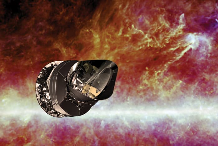
The Planck mission has produced a map of the cosmic microwave background at higher resolution than ever before. Peter Coles explains its implications for our understanding of the universe

On Saturday 19 October 2013 the instruments and cooling systems on the European Space Agency’s Planck spacecraft were switched off, marking the end of the scientific part of the Planck mission, after more than four years of mapping the cosmic microwave background. A day later, in preparation for a final shutdown command, a piece of software was uploaded that would prevent the spacecraft systems from ever being switched on again so that the onboard transmitter would never cause interference with any future probes. At this point Planck had already been “parked” indefinitely in a “disposal” orbit, far from the Earth–Moon system, having been nudged off its perch at the 2nd Lagrangian Point (L2) in August 2013 by a complicated series of spacecraft manoeuvres. These preliminaries having been completed, on 24 October 2013, at 12.00 GMT, a final instruction was successfully transmitted that shut down Planck for good. The Planck spacecraft will continue to orbit silently in the Sun’s gravitational field for the foreseeable future.
But although this is the end of the Planck mission, it is by no means the end of the Planck era. Vast amounts of data still need to be fully analysed and key science results are still in the pipeline. The numerous maps, catalogues and other data products will be a priceless legacy to this generation of cosmologists, and no doubt many future generations. Nevertheless, this seems a good time to step back a little and try to form some sort of perspective on what the mission might mean for cosmology in the longer term. In this article, I’ll try to do this by reflecting on what Planck was actually all about, asking what we have really learned from it, pondering what its scientific legacy might be, and suggesting what might come after it.
What was Planck?
The serendipitous detection of the cosmic microwave background (CMB) radiation in the 1960s provided the first direct evidence that the universe began in a hot Big Bang and led to its discoverers, Arno Penzias and Robert Wilson, being awarded the Nobel Prize for Physics in 1978. In the early days of CMB science, however, all that was known about the radiation was that its temperature is about three degrees above absolute zero, that it is of roughly black-body form (consistent with having been produced in thermal equilibrium with matter), and that it is approximately uniform in all directions on the sky. Theorists realized that the current low temperature is the result of the expansion of the universe and that the black-body radiation had actually been produced at a much higher temperature, at a time when the universe was filled with a plasma of ionized material that scattered radiation very effectively and was therefore opaque.
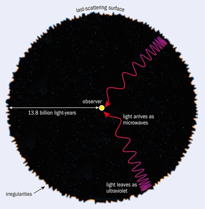
As the universe expanded and cooled, it would have undergone a relatively sharp transition when electrons and ions would have combined to form atoms, at which point the universe became transparent to radiation. This transition mirrors the behaviour of a star like the Sun, in which the matter temperature falls off with distance from its centre. Inside a star the matter is ionized and opaque; outside it is neutral and transparent. The sharp change in the optical properties of stellar matter happens at a temperature of a few thousand degrees, which is why stars have a well-defined surface temperature of that order. The CMB was produced when the entire universe was at a similar temperature to that of the surface of a star. Looking out over cosmological distances we see back to this epoch; we can’t see further because beyond the “last scattering surface”, the universe is opaque (figure 1).
Just as astrophysicists can probe the opaque interior structure of stars by studying oscillations in the surface layers – a technique called stellar seismology – so cosmologists can probe the physics of the early universe using variations in the temperature of the CMB across the sky produced by oscillations in the primordial plasma. These oscillations are of a similar form in both cases – acoustic waves (although the wavelength is much longer in the cosmological setting than in the case of a star).
The basic theoretical framework of the Big Bang assumes the Cosmological Principle – that the universe is homogenous and isotropic. Even the most cursory observation tells us, however, that the universe is not like that, but rather lumpy, which means that any satisfactory cosmological model must explain where all the lumps came from. Our basic explanation for the lumps has not changed since the late 1960s: small initial irregularities in the distribution of matter got progressively amplified by the action of gravity as the universe expanded, eventually forming the rich cosmic web of structure we see today. These initial perturbations should manifest themselves as the variations theorists expect to see in the temperature of the CMB.
The simplest way of thinking about the initial perturbations is to consider the name Big Bang. The existence of a “bang” requires there to be acoustic waves, which are variations in the density and pressure of the medium supporting them. In the absence of such variations there cannot really be a “bang”; a completely uniform universe would really have been born in a Big Silence. If our view of how cosmic structure forms is correct, these primordial acoustic waves must have existed, therefore the universe must have been born in a bang.

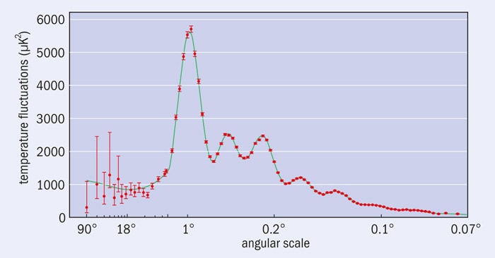
The predicted “ripples” in the temperature of the CMB were not discovered until the early 1990s, when their large-scale variation was detected by the Differential Microwave Radiometer instrument on the Cosmic Background Explorer (COBE), a discovery that led to the award of the Nobel Prize for Physics to John Mather and George Smoot in 2006. COBE only detected the low-frequency part of the “sound” of the Big Bang – those acoustic waves with physical wavelengths that correspond to patches of sky larger than 10° or so. However, it led to the development of many other studies, such as the balloon-borne Boomerang and Maxima experiments, which sought to obtain more information about the higher-frequency content so as to map the CMB sky with greater angular resolution. Then, starting in 2003, a team of researchers used data from the Wilkinson Microwave Anisotropy Probe (WMAP) to map the whole sky over a wider range of microwave frequencies, establishing in the process a nearly complete spectrum of the sound of the Big Bang (figure 2).
Although it was in its planning stages before WMAP, Planck can be seen as a natural successor to WMAP by being more sensitive and having an improved angular resolution, which enabled it to see even shorter-wavelength acoustic ripples than WMAP could. It also had a wider range of receivers that made it better able to distinguish between the true CMB and other sources of radiation from, for example, our own galaxy, that might pollute the cosmic signal.
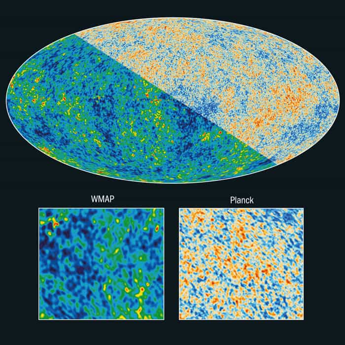
As it turned out, Planck was well up to the task of measuring the CMB spectrum over a huge dynamic range, providing results that were broadly compatible with WMAP but extending to much shorter wavelengths (figures 3 and 4).
So what are the main results from Planck? There are too many to discuss them all in detail – the science release in January 2013 resulted in more than 30 publications and different people will consider different things important. Here is a brief discussion of the three topics that interest me the most.
Cosmology by numbers
Cosmology is an unusual subject in many ways, not least because it appears to be done backwards compared with other branches of physics: instead of setting the initial conditions for an experiment and seeing how it develops, we have to infer how the great cosmic experiment that is our universe started from what we can observe it to have produced. The reason for this is that the Big Bang theory is incomplete. Based on our poor current understanding of how matter behaves at the high temperatures and densities we think occurred much earlier than the plasma phase, researchers are simply unable to predict from first principles precisely how the universe began. Indeed, the equations we use fall apart entirely at the very beginning because of the existence of an initial “singularity” at which the density and temperature become infinite.
This difficulty means that, although we can derive a system of equations, based on Einstein’s theory of general relativity, to describe the universe’s evolution in general terms, this system has a family of solutions corresponding to different initial conditions. We have no way of knowing which, if any, of these solutions corresponds to the universe we happen to live in. We are therefore unable to proceed by reason alone and are forced to seek observational clues.
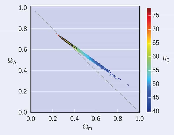
Fortunately, it turns out that we can describe the entire family of possible Big Bang universes in a relatively simple way using a set of (dimensionless) parameters that, at least in principle, we can measure observationally. Many of these parameters can be determined more or less directly from the CMB. For example, the “matter” density is expressed via a parameter called Ωm, which includes both the ordinary baryonic matter from which atoms are made as well as neutrinos and the exotic dark matter that seems to be required by various astrophysical observations. We often need to consider these components separately but for the following discussion it suffices to lump them all together.
Another dimensionless parameter, called ΩΛ, describes a dark-energy component whose origin we don’t understand at all but which, in its simplest incarnation, is related to the cosmological constant term, Λ, introduced by Einstein into his general theory of relativity, way back in 1916.
In this theory of gravity, the matter and dark energy expressed by the previous two parameters determine the curvature of space–time, expressed by another parameter, k. This parameter governs not only the geometry of the universe but also its dynamical evolution. If the curvature is zero then space is “flat” (i.e. Euclidean); in this case Ωm + ΩΛ = 1 so that, in the absence of a cosmological constant, the density of matter Ωm = 1.
In a more general case, the curvature can be either positive (corresponding to a closed spatial geometry, such as a 3D version of the surface of a sphere) or negative (an “open” universe with a hyperbolic geometry such as that of a 3D “saddle”, which is admittedly rather hard to visualize).
Again looking at the case in which ΩΛ = 0, the future evolution of the universe is entirely determined by Ωm. If Ωm > 1 then its current expansion will decelerate, eventually halt and go into reverse; such a universe will recollapse in a Big Crunch. If Ωm < 1 the expansion will continue forever. A dark-energy or cosmological-constant contribution acts to accelerate the expansion of the universe, so models with a large value of ΩΛ typically experience runaway expansion in the future.
There are more parameters than these of course. There is also the Hubble constant, which describes the current expansion rate of the universe, and others relating to, for example, the densities of different types of matter. Minimal versions of the Big Bang model have about half a dozen free parameters, but extended versions have many more, not all of which are independent. I don’t have space to discuss all of them, however, so in the following I’ll just focus on these basic ones.
The existence of free parameters means that the theory is a bit of a moving target; they represent a barrier to direct testing of the theory because they can be tweaked to accommodate new measurements. However, the more precisely we can estimate their values the more we can reduce this wiggle room and subject the overarching framework to critical tests.
In 1994 George Ellis and I wrote a review article for Nature (370 609) in which we tried to weigh up all the available evidence about Ωm. This parameter basically measures the mean density of the universe and it is possible to estimate this in many ways, including galaxy clustering, galaxy and cluster dynamics, large-scale galaxy motions and gravitational lensing. Many of these techniques were in their infancy at the time but, based on the available evidence, we concluded that the value of Ωm was between about 0.2 and 0.4.
This verdict was somewhat controversial because of a theoretical predilection for a picture of the early universe, known as cosmic inflation, in which the expansion of the universe expands by an enormous factor, perhaps 1060, very soon after the Big Bang. This stretches the universe so that it is expected to appear very flat; k is driven towards zero to very high accuracy. At the time there wasn’t much direct evidence for a cosmological constant, and in the absence of this, a flat universe would require Ωm = 1. As it turns out, the subsequent development of these techniques has not changed our basic conclusion that Ωm = 0.2–0.4. The last 15 years or so have, however, seen two stunning observational developments that we did not foresee at all.
Beginning in the late 1990s, two major programmes, the Supernova Cosmology Project led by Saul Perlmutter and the High-z Supernova Search Team led by Adam Riess and Brian Schmidt, exploited the behaviour of a particular kind of exploding star, type Ia supernovae, to probe the geometry and dynamical evolution of the universe. The measurements indicate that distant high-redshift supernovae are systematically fainter than one would expect (based on extrapolation from similar nearby low-redshift sources) if the universe were decelerating. The results are sensitive to a complicated combination of Ωm and ΩΛ but they strongly favour accelerating-world models and thus suggest the presence of a non-zero cosmological constant, or some form of dark energy. The leaders of these supernova studies were awarded the Nobel Prize for Physics in 2012.
The supernova searches were a fitting prelude to the stunning results that emerged from WMAP in 2003. The CMB is perhaps the ultimate vehicle for classical cosmology. When you look back to a period when the universe was only a few hundred thousand years old, you are looking across most of the observable universe. This enormous baseline makes it possible to carry out exquisitely accurate surveying. The observed spectrum of the temperature variations displays peaks and troughs that contain fantastically detailed information about the basic cosmological parameters described above (and many more). Earlier CMB experiments, especially WMAP, established a basic framework called the concordance cosmology. Planck not only confirmed this picture but made it much more precise, pinning down the free parameters to unprecedented accuracy (figure 5).
The increasing precision of cosmological-parameter estimates has tightened up the theoretical slack in the Big Bang model, but not without generating a certain amount of tension. Combining the CMB measurements with other data (such as the supernovae or measurements of large-scale structures) does seem to move the best-fit values slightly away from where they would sit if derived from the CMB alone. However, the statistical evidence for discordance among the parameters – for major departures from the standard Big Bang model – remains marginal, at least for the time being.
The confirmation and refinement of the concordance cosmology is a great achievement, on a par with the establishment of the Standard Model of particle physics. But there is more to cosmology than increasing the precision of cosmological-parameter estimates. We also need to ask if we can discover evidence of anything outside our standard view of the cosmos.
Non-Gaussianity
One important topic is the “non-Gaussianity” of the CMB, because the simplest theories of cosmological inflation predict the generation of small-amplitude irregularities in the early universe that imprint themselves upon the observed radiation pattern. These irregularities are essentially in the form of acoustic waves, so in a very real sense it is inflation that put the “bang” in Big Bang and was thereby responsible for creating galaxies and the large-scale structure of the universe. In the standard cosmological model, these acoustic waves form a statistically homogeneous and isotropic random field. Technically, this means that the perturbations have probability distributions that are invariant under translations and rotations in 3D space. Such fluctuations appear in inflationary cosmology in a manner essentially identical to the zero-point fluctuations that arise from the quantized harmonic oscillator problem and that are well known to be described by Gaussian statistics.
According to the theory of cosmological inflation, the dynamics of the early universe were dominated by a hypothetical scalar field called the inflaton. Assuming the fluctuations are small in amplitude, the scalar field evolves according to the same sort of dynamical equation that also describes, for example, a massive body falling through the air. Eventually such a body reaches a terminal velocity, which is defined by the balance between gravity and air resistance (drag) but is independent of how high and at what speed it started falling. The problem is that if you want to know where a body moving at terminal velocity started falling from, you’re stumped: all dynamical memory of the initial conditions is lost when terminal velocity is reached.
The problem for early-universe cosmologists is similar. In the context of cosmology there is a “slow-rolling” regime in the evolution of the inflaton field that is analogous to drag-limited motion of a falling body; in such a regime the universe enters a near-exponential phase of accelerated expansion, which causes it to inflate. In this phase the small-amplitude Gaussian quantum fluctuations in the scalar field become CMB fluctuations, which are Gaussian to a very high precision. If everything we measure is consistent with having been generated during a simple slow-rolling inflationary regime, then there is no way of recovering any information about what happened beforehand because nothing we can observe today will remember it. The early universe will remain a closed book forever. On the other hand, if inflationary dynamics were a bit more complicated (such as if there were multiple scalar fields rather than just a single inflaton) the fluctuations need not be so accurately Gaussian.
Before Planck, all statistical studies of CMB fluctuations had generated results consistent with Gaussian fluctuations. One of the most important things that the Planck collaboration has been looking for is evidence of non-Gaussianity that could be indicative of primordial physics more elaborate than that involved in the simplest inflationary models described by the slow-rolling solution.
Because we don’t know a priori whether any of these ideas are correct, we cosmologists encode the level of non-Gaussianity in a parameter called ƒNL and have designed sophisticated statistical tests to estimate it from observed data. By far the most precise measurements of this quantity have come from Planck; the value is ƒNL = 2.7 ± 5.8 which, within the error bars, is clearly consistent with zero. If this limit doesn’t look impressive, note that ƒNL is defined as a quadratic correction to an assumed Gaussian component. In essence we are modelling the CMB in the form a + bx + cx2, and we already know a (the mean temperature) and b (the amplitude of the Gaussian component) and want to measure the value of c (which is ƒNL), which represents the size of a non-Gaussian contribution. The typical temperature fluctuations seen on the CMB sky are about one part in 105 of the mean temperature (about 2.73 K); quadratic terms are therefore of an order 10−10, so the upper limit on the level of non-Gaussianity allowed by Planck really is minuscule; it is Gaussian to a few parts in a hundred thousand. This is one of the reasons why some people have described the best-fitting model emerging from Planck as the Maximally Boring universe.
Perhaps this is a signal that we are approaching the limit of what we can learn about inflation in particular, or even the early universe in general, using the traditional techniques of observational cosmology?
Cosmic anomalies
Although Planck seems to have closed the window on the possibility of probing the early universe using non-Gaussianity (by not finding any), it has left another window very firmly open. As well as providing the strong basis for the concordance cosmological model discussed above, the WMAP data also provided some tantalizing hints of anomalous behaviour in the CMB sky that can’t be accounted for by the standard cosmology.
One way of looking at how cosmology works is to think of it as an enormous exercise in data compression: Planck’s raw map of the CMB sky consists of millions of pixels each measured at nine different wavelengths. From this, one can extract the spectrum shown in figure 3, which consists of a few dozen data points plotted on a graph, and from the spectrum we can extract a handful of very precise parameter estimates. This data compression is possible because the data are assumed to be described by a statistically homogeneous and isotropic Gaussian random field, which means that the spectrum contains all the relevant information in the map. All other degrees of freedom in the data are irrelevant (or “non-informative”) for cosmology.
This compression scheme only works, however, if the underlying assumption is correct. As I have explained, upper limits on the particular form of non-Gaussianity described by ƒNL are consistent with this assumption but there could be other departures that we don’t know how to characterize. These would be missed by the standard analysis pipeline, so it’s important to check the data rigorously with as many tools as possible to check we haven’t discarded any important clues.
The possible anomalies detected by WMAP included a curious “cold spot” that appears to be colder than one would expect on the basis of Gaussian statistics. WMAP also revealed an unexpected alignment between fluctuation patterns on large angular scales, chiefly between the quadrupole (90°) and octupole (45°) modes corresponding to the first two points on the left of figure 2. And finally, there was a marked asymmetry in statistical properties of the observed CMB between the hemispheres north and south of the ecliptic plane.
Opinions about these WMAP anomalies differ among cosmologists, with many thinking that they are just systematic artefacts of the experimental procedure but others convinced that they may provide clues to physics beyond the standard model (such as deviations from the cosmological principle). Intriguingly, all the anomalies found by WMAP are also present in the Planck data; there remains no consensus on their significance.
What next?
In summary, what Planck has done is to confirm and render more precise a standard view of cosmology that already existed rather than provide dramatic and revolutionary new insights. It has increased the precision of cosmological-parameter estimates and in so doing has given us a detailed quantitative description of the geometry, expansion rate and energy budget of the universe. It has provided strong evidence to support the simplest theory of cosmological inflation and also, by placing strong constraints on the level of primordial non-Gaussianity, excluded more exotic variants of the inflationary idea. It has also confirmed the existence of various anomalies found by WMAP though not really confirmed whether they provide significant evidence of physics beyond the standard model of cosmology.
So what comes next? The most obvious answer to that question is CMB polarization. The analyses of Planck data published so far focus exclusively on the variation in temperature (effectively the intensity) of the CMB across the sky. However, theory predicts that the radiation field should be partially polarized as a consequence of scattering from electrons in the primordial plasma. Measuring the polarization of the CMB is a formidable technical challenge, which explains why it will take the Planck collaboration much longer to analyse the data than in the case of the intensity alone, but promises rich rewards if it can be done. Among other things, the polarization of the radiation field depends in a particular way on the existence of primordial gravitational waves, a key prediction of inflationary theories.
The first polarization data from Planck will not be available until later this year at the earliest, but such is the importance of this aspect of the CMB that there are already missions planned as successors to Planck, such as one from the European Space Agency called PRISM.
Although we have learned a very great deal from Planck and other complementary studies, there is still a great deal about the state of the universe that we misunderstand at a fundamental level. In particular we want to know if dark matter and dark energy are real or just manifestations of something wrong with the applicability of general relativity on cosmological scales. Only time, and more data, will tell.