From proteins to DNA, knotted structures are present in many vital molecules. Understanding what these knots do is difficult because our best theories still struggle to tell complex knots apart. But, argues Davide Michieletto, with advances in AI, that could be about to change

Any good sailor knows that the right choice of knot can mean the difference between life and death. Whether it hoists the sails or secures the anchor, a rope is only as good as the knot that’s tied in it. The same is true, on a much smaller scale, for many of the molecules that keep us alive.
Proteins are essential building blocks for all living things, and these long chains of amino acids form complex 3D shapes that allow molecules to fit together. For a long time, it was thought that while proteins can be highly tangled, they could not form knots under normal conditions, as this would prevent the proteins from being able to fold. But in the 1970s researchers found many topologically knotted proteins, in which their native structures are arranged in the form of an open knot.
As it happens, despite proteins (and even DNA) having “open” curves, knots can still form and affect their function. Indeed, they comprise about 1% of proteins in the Protein Data Bank. Unlike a rope or string, each protein of this type has a characteristic knot (figure 1). The largest group of knotted proteins is the SPOUT family of enzymes (which make up the second largest of seven structurally distinct groups of methyltransferases enzymes), all but one of which are knotted in a “trefoil” of three overlapping rings.
1 Knots for life
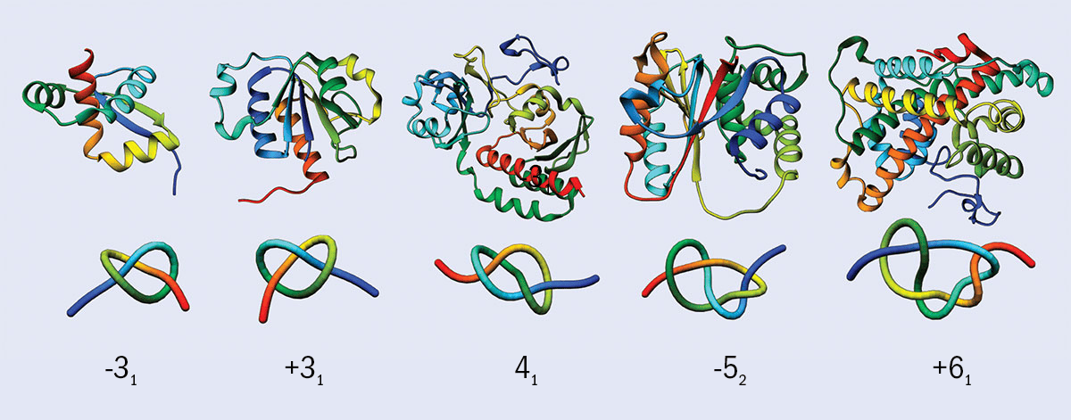
Some proteins form well-defined knotted structures, as shown above, where the lower image shows a simplified view of each molecule. The number below each image indicates the number of times the protein crosses itself and the + and – indicate that they are mirror images. The –31 and +31 for example are mirror image instances of the “trefoil” knot. Proteins form “open knots” because their two ends don’t join up. However, it is often still possible to define a knotted structure in the molecule.
This discovery raised many questions, such as how and why these knots form, what is the mechanism of their folding, and what role this might play on a functional level. There is some evidence that knotted proteins are more resistant to extreme temperatures, but scientists still do not know how abundant knots are in molecular structures or exactly how knotting affects their biological function.
The trouble is that when we try to apply what we know about knots to questions in biology and soft matter, we come up against a mathematical problem that’s been confounding scientists for over a century.
A tangled history
The origins of modern knot theory are often traced back to a famous experiment that was performed more than 150 years ago – not with ropes or string, but with smoke.
In 1867 Peter Guthrie Tait invited his friend and fellow physicist William Thomson (later Lord Kelvin) to travel from Glasgow to Edinburgh to witness a demonstration where he generated pairs of smoke rings. To Kelvin’s surprise, these rings were remarkably stable, travelling across the room and even bouncing off each other as if they were made of rubber. A smoke ring is a “vortex ring” in which the aerosols and particulates are rotating in small concentric circles, and this motion gives the ring its stability.
At the time, it was widely believed that the universe was pervaded by a space-filling substance dubbed “aether”, through which gravitational and electromagnetic radiation propagated. Kelvin reasoned that atoms might be made from stable vortices, like smoke rings, in this aether. He further argued that knots tied in aether vortex rings could account for the different chemical elements.
The vortex theory of atoms was incorrect, but knot theory continues to this day as a branch of mathematics
Tait was intrigued by Kelvin’s theory. Over a period of 25 years, and with the help of the Church of England minister Thomas Kirkman, American mathematician Charles Little and James Clerk Maxwell, Tait produced a table of 251 knots with up to 10 crossings (figure 2). The vortex theory of atoms was incorrect, but knot theory continues to this day as a branch of mathematics.
2 Order and disorder
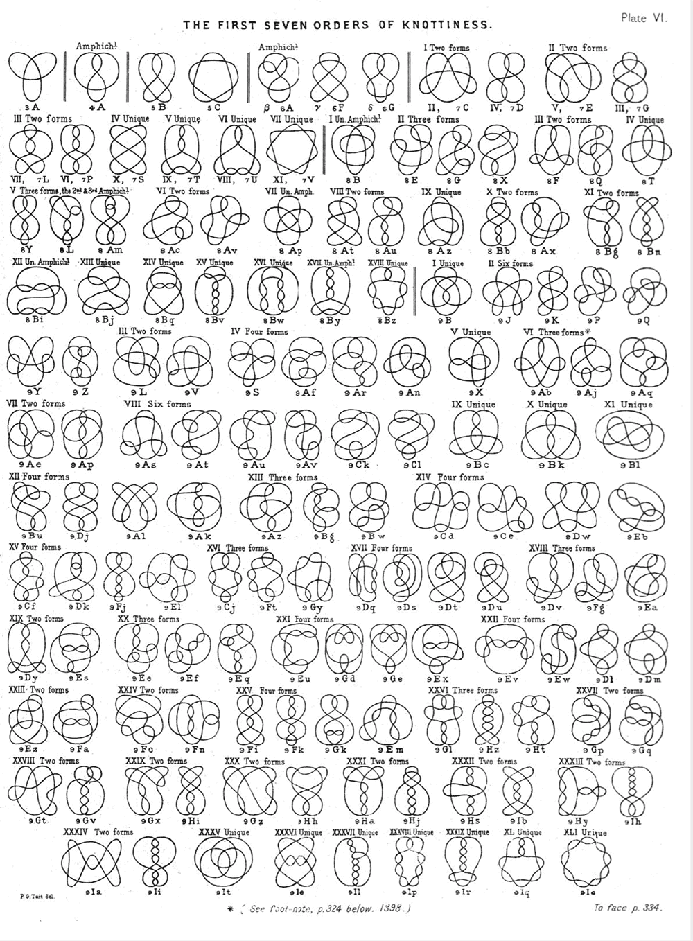
Peter Guthrie Tait and other early knot theorists spent years compiling a comprehensive list of knots. The above image is extracted from their table of knots up to seven crossings – “the first seven orders of knottiness”.
Spot a knot
For Tait and his fellow theorists, the classification of knots was painstaking work. Every time a new knot was proposed, they had to check that it was unique using drawings and geometric intuition. Tait himself wrote that “though I have grouped together many widely different but equivalent forms, I cannot be absolutely certain that all those groups are essentially different from one another”. Indeed, in 1974 Kenneth Perko showed that two entries in the original table are actually the same knot – these are now known as the “Perko pair” (Proc. Amer. Math. Soc. 45 262).
If you need any more convincing, my student Djordje Mihajlovic has developed an online game called “Spot a Knot” where the goal is to spot equivalent knots from pictures (figure 3). Even after years of researching knots, I often get it wrong. To earn a spot in the table, a knot must have a unique topology, meaning that it cannot be deformed into any other known knot without being broken. As the Perko pair and Mihajlovic’s game show, proving that two knots are different is easier said than done. Remember that topology studies the properties of spaces that do not change if they are deformed smoothly; to a topologist, a mug is equivalent to a doughnut because one can be massaged into the other without losing the inner hole.
3 Brain teaser
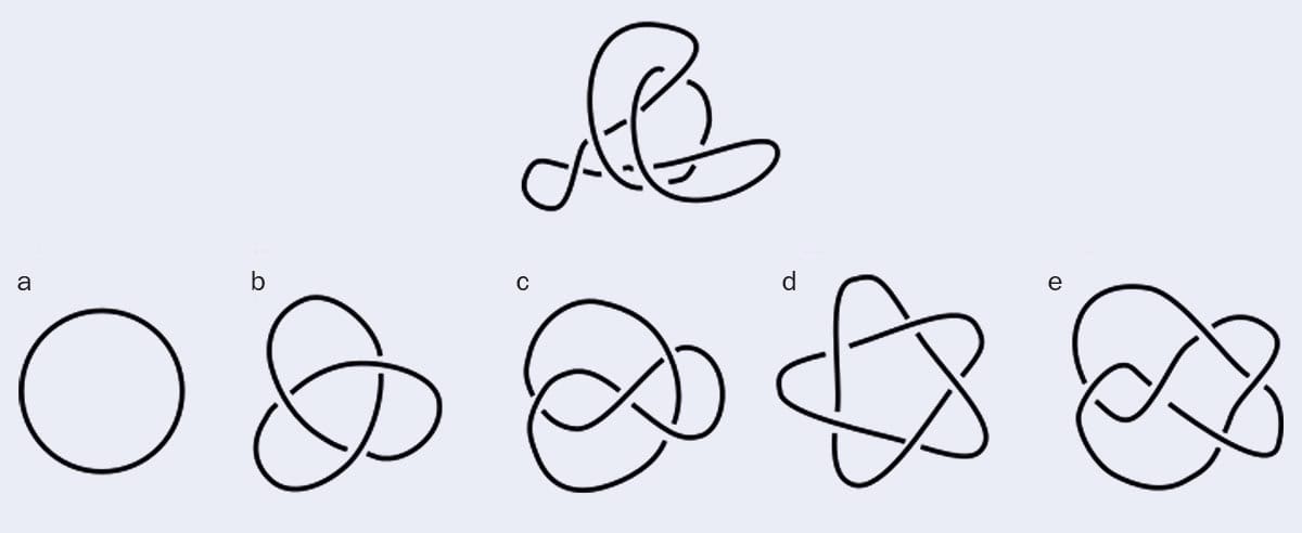
To illustrate the difficulty of identifying knots, Djordje Mihajlovic – a PhD student at the University of Edinburgh – developed an online game called “Spot a Knot”. One question is reproduced above. Does the top image correspond to a, b, c, d or e?
As scientists learned more about the structure of the atom, the vortex atom model was gradually abandoned. A final blow came in 1913 when Henry Moseley showed that chemical elements are differentiated not by their topology but by the number of protons in the nucleus.
In knot theory, quantities that describe the properties of knots are called “invariants”. The dream of knot theorists is to find a quantity like the proton number that can classify any knot based on its topology. Such a “complete invariant” would yield a unique value for every unique knot, and wouldn’t change if the knot were smoothly deformed.
The knotted strands of life
A recipe for such a topological invariant could be something like this: “Walk along the knot and label each of the n crossings with numbers 1, 2, 3, …, 2n (you will traverse the knot twice). If the label is even and the line is an overcrossing, then change the sign of the label to minus (figure 4). At the end, each crossing will be labelled by a pair of integers, one even and one odd. The series of even integers is a code for the knot.” This recipe is called the Dowker–Thistlethwaite code, first proposed in 1983 (Topology and its Applications 16 19) (figure 5).
The Dowker–Thistlethwaite code can classify many simple knots, but like every other method that’s been proposed, it isn’t a complete invariant. The first knot invariant was proposed in 1928 by James W Alexander and called the Alexander polynomial. Since then, many others have been developed, but for each one, a case has been found where it fails to make a unique classification.
Taking a walk
The Alexander polynomial belongs to the family of so-called “algebraic invariants”. It is computed by constructing a matrix with as many rows and columns as there are crossings in the knot, and taking its determinant. Algebraic invariants are constructed from a 2D projection of the knot. This is a bit like a shadow, but one where we can discern which part of the loop is on top each time it crosses itself.
Soft-matter physicists like myself, however, want to classify the knots in molecules like proteins and DNA, which are 3D and constantly jostled by thermal energy. Reducing these molecules to 2D projections erases spatial features that may be crucial to their function.
An attractive alternative for characterizing molecules is “geometric invariants”. These are calculated by traversing the knot in 3D and computing some geometric property, such as the curvature, along the route.
One such invariant that I am fond of is the “writhe”, which was introduced by Tait. Writhe can be measured on a 2D projection by counting the “over” and “under” crossings and subtracting one from the other (figure 4b).
4 Over and under
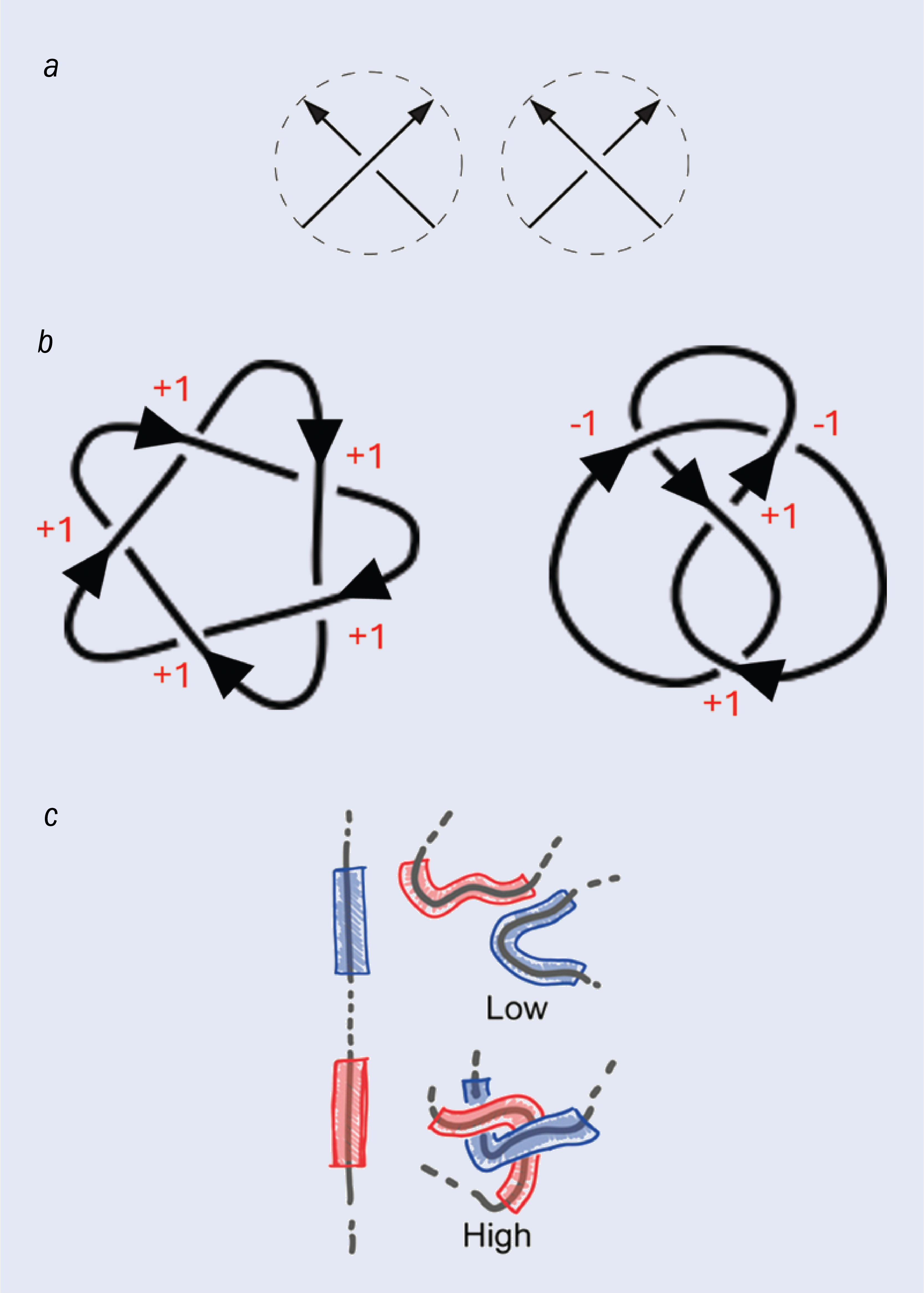
One way to tell the difference between knots is to measure the “writhe”, which quantifies the amount of twisting. (a) Each time the knot crosses itself, the crossing can be characterized as either an overcrossing (left) or an undercrossing (right). The writhe is calculated by subtracting the number of undercrossings from the number of overcrossings.
(b) How the writhe is calculated for two knots – the cinquefoil knot (left), which has a writhe of +5, and the figure-eight knot (right), which has a writhe of 0.
(c) The writhe can also be calculated as a geometric quantity on a 3D molecular knot such as a protein. The geometric writhe can be calculated over the entire knot or as a local quantity between short, adjacent strands. A high value of the “local writhe” indicates that the strands are entangled with each other. Davide Michieletto and colleagues showed that a neural network trained on the local writhe characterizes knot topology with high accuracy.
However, writhe can also be computed as a geometric quantity. Imagine walking along a 3D knot, such as a protein, and at each step writing down an estimate of the writhe by counting the crossings you can see. At the end of your journey, the average of these numbers will yield the true value of the writhe. Unfortunately, writhe isn’t a complete invariant. In fact, like its algebraic counterparts, no geometric invariant has ever been proved to uniquely classify all knots.
In 2021 Google DeepMind’s AlphaFold artificial-intelligence programme solved a problem that had been evading scientists for decades – how to predict a protein’s structure from its amino acid sequence (Nature 596 583). The function of proteins depends on their 3D structure, so AlphaFold is a powerful tool for drug discovery and the study of disease.
The question we asked ourselves was: could AI do the same for the knot invariant problem?
Wriggle and writhe
Using AI to classify knots has been explored by previous researchers, most recently by Olafs Vandans and colleagues of the City University of Hong Kong in 2020 (Phys. Rev. E 101 022502) and Anna Braghetto of the University of Padova and team in 2023 (Macromolecules 56 2899). In those studies, they treated the different knots like strings of beads and trained a neural network to identify them by giving it the Cartesian coordinates and, in the latter case, the vector, distance and angles between the beads.
5 Encoding knots

The Dowker–Thistlethwaite notation is a knot-invariant first proposed in 1983. This method assigns a sequence of integers to a knot by traversing it twice and assigning a number to each crossing, as shown in the image. The final sequence characterizes the knot.
These researchers achieved high accuracies, but only for the five simplest knots. We wanted to extend this to much more complicated topologies, while also simplifying the neural network architecture and using a smaller training dataset.
To do this we took inspiration from nature. In our bodies, knots in DNA are untangled by specialist enzymes called topoisomerases. These enzymes cut and reattach DNA strands and they can effectively smooth out knots despite being about a thousand times smaller than a DNA molecule.
We hypothesized that the topoisomerases can sense some local geometric property that allows them to locate the most tightly knotted part of the DNA molecule. We tried to do this ourselves using various quantities including the density and the curvature. In the end our results led back to the beginning – to Tait and his geometric writhe.
We decided that giving our AI the local writhe would give it the best chance to successfully identify complex knots
As well as calculating writhe over an entire knot, we can also measure it as a local quantity that tells us how much segment x is entangled with nearby segment y (figure 4c). We found that local writhe is a remarkably effective way to locate knotted segments in long, looping molecules (ACS Polymers Au 2 341). Based on this result, we decided that giving our AI the local writhe would give it the best chance to successfully identify complex knots.
Armed with our theory, we began building a neural network to test it. To start, we generated a training dataset by simulating the thermal motion of the five simplest knots, extracting tens of thousands of conformations (figure 6a).
Make or break: building soft materials with DNA
We then trained two neural networks: one using the Cartesian coordinates of the knots and one using the local writhe. In each case, we supervised the AI, and used a subset of our training dataset to tell the neural networks what type each of the knots was. To test our method we asked the neural networks to classify conformations of these simple knots that they hadn’t seen before.
When the AI was trained on the Cartesian coordinates on a simple neural network, it made a correct categorization only four times out of five, similar to what Vandans and Bragetto found. This is probably better than the score most of us would get in the Spot a Knot game, but it’s still far from perfect.
However, when the neural network was trained on the local writhe, the difference was staggering: it could correctly classify the knots with more than 99.9% accuracy.
Tougher challenges
Though I was surprised by this result, the identification of the five simplest knots is relatively trivial, and can be achieved using existing invariants (or an extremely eagle-eyed Spot a Knot player).
We decided to give the neural network a much trickier challenge. This time it would only have to classify three knots rather than five, but we had chosen them carefully: the Conway knot, the Kinoshita–Terasaka (KT) knot and the unknot – the simplest of all knots. The first two have 11 crossings, and are “mutants” of each other because they are identical except in one region where the knot is “flipped”. They share many knot invariants, and they also share some invariants with the unknot.
6 Spot the difference
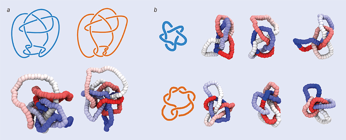
A complete knot invariant shouldn’t change when a knot is smoothly deformed, but should return a different result for topologically distinct structures. Do the two pictures in a show the same knot? It’s often difficult for human intuition to tell knots apart. In fact, the two pictures show two slightly different structures – the Conway and Kinoshita–Teresaka knots. Because it’s difficult to tell them apart, these two knots can be used to test a knot-characterization neural network.
The images in b show different configurations of two knots – the 51, or cinquefoil knot (above) and the 72 knot (below). In Davide Michieletto and colleagues’ work on neural networks, the cinquefoil was part of the first training dataset and the 72 was included in the larger dataset.
What we discovered is that the Conway and KT knots were indistinguishable for a neural network trained on Cartesian coordinates but they could be identified 99.9% of the time by the neural network trained on the local writhe.
The final test was to apply this training to a much larger pool of knots. We ran simulations of 250 types of knots, with up to 10 crossings (figure 6b). When the neural network was trained with the Cartesian coordinates it made a correct classification only one time out of five. By contrast, our best local-writhe-trained neural network could classify all 250 knots in a matter of seconds with 95% accuracy, much better than any other algorithm or single topological invariant (Soft Matter 20 71).
A final twist
Without knowing anything about knots or knot theory, our neural network had taught itself to do something that has long evaded human intuition. In fact, we are still working to open the “black box” and understand what exactly it discovered.
We have found that to distinguish the five simplest knots, the neural network takes every set of pairs of points on the knot and multiplies the writhe at the two points together. What’s intriguing is that this quantity is equivalent to an existing invariant called the “Vassiliev invariant of order two”.
Vassiliev invariants are computed by multiplying pairs, triplets, quadruplets, up to n-tuples of the local writhe matrix. Incidentally, the Vassiliev invariant of order 2 is also the coefficient of the quadratic term of the Conway polynomial, the algebraic invariant we saw earlier. It’s been proposed, though never proved, that the complete set of Vassiliev invariants, which can be computed as an integral, is the long-searched-for complete invariant.
We were excited to find that as it’s presented with more complex knots, the neural network adapts by computing Vassiliev invariants of higher order
We were therefore excited to find that as it’s presented with more complex knots, the neural network adapts by computing Vassiliev invariants of higher order. For instance, to uniquely classify the first five knots, the neural network requires only the degree two Vassiliev invariant. But for the 250-knot dataset, it may compute the Vassiliev invariants up to order three or four.
Geometric and algebraic invariants are computed using very different mathematics, so it’s exciting that AI can discover connections between them, and this brings us a step closer to discovering a complete invariant.
Knotting else matters
In only three years, AlphaFold has generated millions of proteins, most of which have yet to be fully studied. In 2023 a group led by Joanna Sulkowska of the University of Warsaw predicted that up to 2% of human proteins generated by AlphaFold are knotted, with the most complex knot found having six crossings (Protein Sci. 32 e4631). The year before, Peter Virnau of the Johannes Gutenberg University Mainz discovered a protein knot with seven crossings in the AlphaFold2 dataset (Protein Sci. 31 e4380). This protein has never been observed experimentally, so it’s possible that even more complex knots are out there.
Knots don’t crop up only in biology; knotted topologies have also been found to influence the thermodynamic and material properties of ice and hydrogels; meaning that in the future, we may use topology to design new materials. We need powerful methods to identify the structural fingerprints of knots in molecules and materials and we hope that our findings will inform this search. Knotting really does matter.
In 2004 three researchers in Canada used their university’s computing cluster to extend the table of knots, first compiled by Tait, up to 19 crossings, identifying more than six billion unique structures (Journal of Knot Theory and Its Ramifications 13 57). Having taken 25 years to create his list, Tait would probably have been shocked to learn that a century later, a machine would be able to extend his work by more than five orders of magnitude, in just a few days.
The biggest outstanding challenge in knot theory remains the search for the elusive complete invariant. Now that we are enabled by AI, the next step forward might take us equally by surprise.