Richard Corfield explains how our understanding of geological time has been revolutionized over the last decade by studying how cyclic variations in the Earth’s orbit are encoded into sediments and rocks

At the start of George Pal’s film of H G Wells’ novella The Time Machine, a dishevelled Rod Taylor stumbles into a dinner party of his friends with a tale to tell. He has been building a time machine that has taken him to the far future where the evil Morlocks battle the gentle Eloi for domination of the Earth. A masterpiece of retro-Edwardian engineering, the device is dominated by a huge spinning disc that controls its movement through time. Push the lever forwards for the future, backwards for the past, and the faster the disc cycles, the faster through time you travel.
If only life were so simple. A handy little time machine would, after all, be the answer to many of the biggest questions in geology. How long ago did something happen? What was its duration? When did it finish? These questions are asked daily by geologists of all flavours – whether they are tracing the evolution of species, trying to work out when a particular range of mountains formed, analysing changes in the Earth’s sea level or deciphering major historical shifts in our planet’s climate.
This latter discipline, which involves using rocks and sediments to elucidate the Earth’s past climate, has become a field of geological research in its own right, known as “palaeoclimatology”. But palaeoclimatology has also started to revolutionize the way that geological time is measured and has given geoscientists of all types an accurate way of calibrating and measuring time. Indeed, by combining this knowledge with periodic variations in the Earth’s orbit, it has become possible to discriminate between geological events with a precision of 1% or better.
The geology game
There are two fundamental approaches to the way that time is measured in the earth sciences: relative and absolute.
Relative time is the province of “stratigraphy”, in which geologists study the layers in rocks. Such “strata” are a feature of sedimentary rocks, which are formed by sediments being deposited, compressed and then hardened over geological time. Rock strata can be laid down in a variety of different environments, for example in deep sea beds or in shallow waters. To the naked eye, rock strata at different depths and locations often look very similar – so how then can they be used to measure relative time? The answer lies with palaeontology: the study of fossils.
The beauty of these preserved remains of former plants and animals is that the evolutionary development of individual “lineages” of fossils is unique – it never repeats. Any particular fossil-containing “biostratigraphic” layer contains fossil fauna that are as distinctive as a fingerprint. Find that fingerprint in other locations and you know that these rocks are the same age. However, there are other ways of matching the ages of sediments and rocks, including one that exploits the fact that the direction of the Earth’s magnetic field has flip-flopped over the course of geological time – sometimes for relatively short intervals of a million years or less and sometimes for much longer periods of up to 100 million years. What this means is that each rock stratum has a magnetization that indicates the polarity of the Earth’s magnetic field at the time the stratum was deposited.
Geologists can identify each successive pair of time periods over which the Earth’s magnetic field first pointed one way and then the other
Using the magnetic polarity of rocks for correlation – a technique known as “magnetostratigraphy” – geologists can identify each successive pair of time periods over which the Earth’s magnetic field first pointed in one direction and then the other. These “polarity chrons” are numbered in order starting from today and increasing into the past, with the dinosaurs going extinct, for example, 66 million years ago during Chron 29. But because there are only two types of magnetic signature – normal or reversed polarity – magnetostratigraphy has to be combined with biostratigraphy (with its unique fingerprint) to identify which chron is which. Combining these chron boundaries with biostratigraphic data, researchers have created what is now known as the geomagnetic polarity time scale, which matches geological events, such as different ice ages, to the flipping of the Earth’s magnetic field (see box).
The geomagnetic polarity time scale
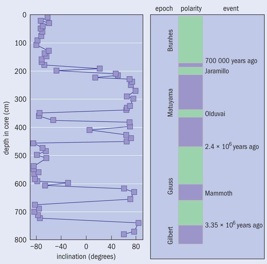 It has been known since the 1920s that the Earth’s magnetic field undergoes periodic reversals, with the most recent of these zones of flip-flopping magnetism (“chrons”) depicted on the above timeline. (Green indicates that the direction, or “inclination”, of the field was opposite to what it is today.) The rocks that were being created in the regions where new crust forms (mid-ocean ridges) took on the magnetization prevailing at the time. These rocks are formed where tectonic plates move apart and lava emerges from the gap between the plates before spreading horizontally along the sea-bed floor. But the magnetic field directions are also encoded at different depths in sediments below the sea bed. So as the sea bed spreads at a more-or-less constant rate of about 1 cm per 1000 years, if you can measure the horizontal distance between chrons on the sea bed it is possible to estimate the time that elapsed between magnetic reversals. And if you match the age of a recently formed region on the sea floor with its corresponding chron in a sediment, you can start assigning dates to chrons – and hence to biostratigraphic boundaries calculated by studying the fossil record.
Gatekeepers of time
The geomagnetic polarity time scale has been a great achievement but essential to its success has been the addition of control points of actual, absolute date. Assigning true chronological ages to rocks is the science of “geochronology” and its father is the New Zealand nuclear physicist Ernest Rutherford. He famously established the principles underlying the radioactive transmutation of elements while working at McGill University in Canada with Frederick Soddy in 1902 and almost immediately realized that the spontaneous decay of radioactive materials could be used to measure the passage of time in the fossil record. As unstable isotopes decay at a particular rate, all we need to do to obtain a natural chronometer is to measure the accumulation of stable daughter products in minerals that had once borne radioactive materials.
Geochronology developed through the 20th century, with various isotope systems being investigated and their decay constants refined, including uranium to lead, uranium to thorium, and neodymium to samarium. But by the 1990s, when the geomagnetic polarity time scale had fully matured, the favoured system was the decay of radioactive potassium-40 nuclei into stable argon-40. The quantity of potassium-40 in a particular rock falls away exponentially with a half-life of about 1.25 billion years, whereas any argon-40 that is created remains trapped within the material. So by measuring the amount of these isotopes in the rock and knowing the half-life of potassium-40, it is simple to calculate the age of the sample.
The “K–Ar technique”, as it is known, can be used on any cores and rock sections that contain potassium-rich minerals, such as glauconites. It has allowed the absolute ages of particular strata of deep-sea cores and outcrops of rocks on land to be determined. It has also been widely used to date hominid fossils found in East Africa, with, for example, the australopithecine ape Lucy – the skeleton of which was discovered in 1974 – being judged to be 3.2–3.4 million years old. Unfortunately, K–Ar dates cannot be applied systematically to all cores and rock outcrops because the relevant minerals required to make the measurements are not necessarily always present.
Age points therefore have to be correlated to different outcrops or cores using indirect methods, such as through biostratigraphic and magnetostratigraphic data. But even with such techniques, there are limitations on the available time resolution, imposed by the relatively long gaps between identifiable dates. So, for example, if two absolute dates are 10 million years apart, then even if we identify 20 different equally spaced biostratigraphic fingerprints in between, the best temporal resolution will then be 500,000 years, which is still a long time. Thankfully, however, a way to address this problem has emerged over the last decade.
Windmills of your mind
The standard methods for constructing geological timescales – based on geochronology, magnetostratigraphy and biostratigraphy – changed drastically in the 1990s with the advent of a new kind of dating technique, known as “astrochronology”. This technique builds on the work of the Serbian astronomer Milutin Milankovic´, who between 1915 and 1940 worked out a mathematical theory for the major climate cycles that occurred towards the end of the Pliocene epoch (which finished 2.6 million years ago) and then throughout the Pleistocene (from that point to 11,700 years ago).
During these cycles, the Earth’s glaciers repeatedly pushed outwards from the poles – sometimes reaching as far as 40˚ either side of the equator – before retreating back and then going out again. Milankovic´ hypothesized that these regular cycles, which reoccurred about once every 110,000 years, were caused by periodic variations in the quantity and distribution of solar radiation falling on the Earth – and that these changes in sunlight were in turn caused by variations in the eccentricity, precession and obliquity of the Earth’s orbit (figure 1).
1 Cycling through history
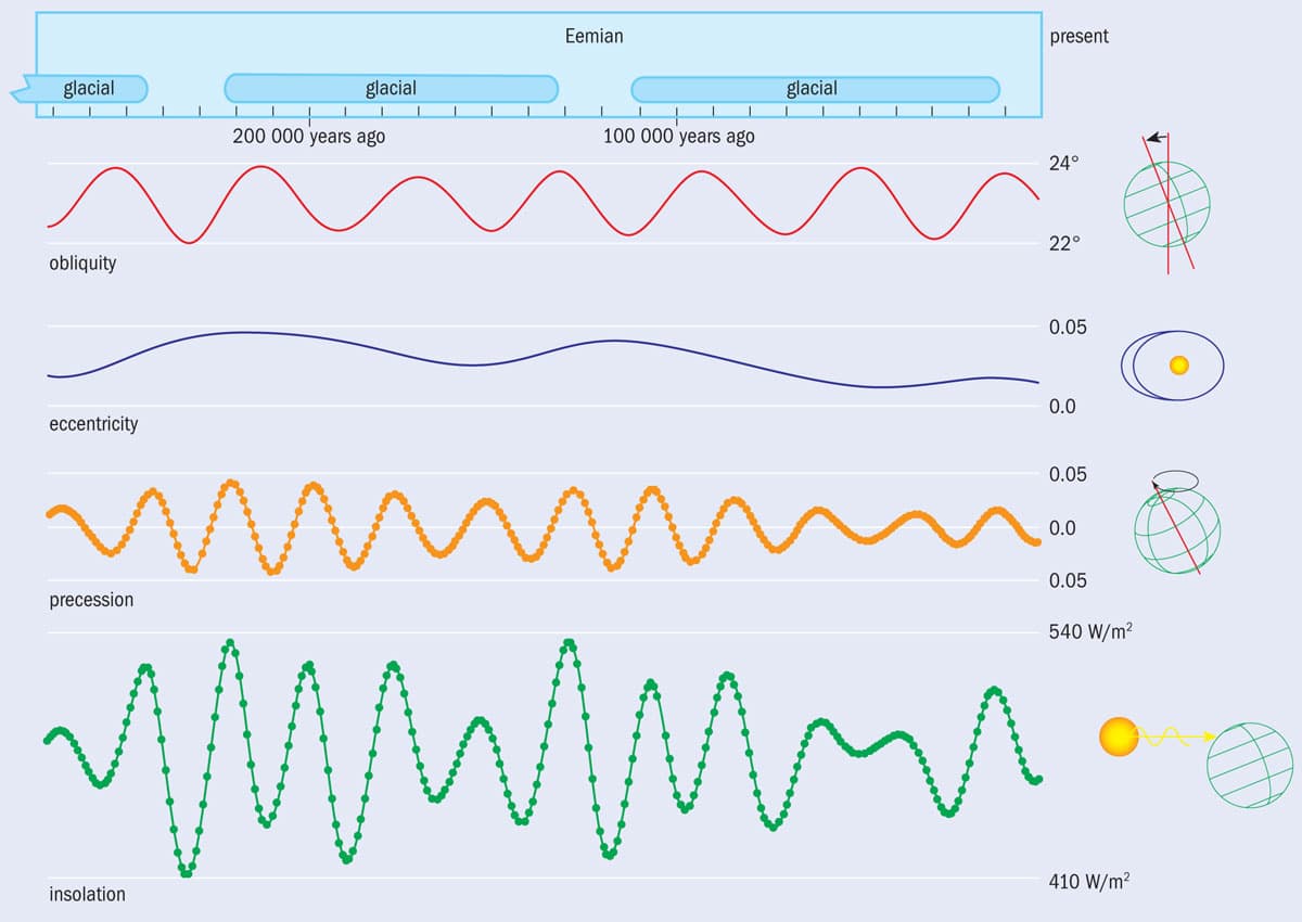
As was first realized by the Serbian astronomer Milutin Milankovic´, the Earth has undergone huge climate cycles each lasting roughly 110,000 years during which time the planet’s glaciers repeatedly pushed out towards the equator before retreating. These cycles were caused by periodic variations in the amount and distribution of sunlight falling on the Earth, which were in turn the result of variations in our planet’s obliquity (tilt), eccentricity (deviation from a true circular orbit) and precession (the poles wobbling about the axis). Shown here are the changes in sunlight falling at an altitude of 65°N, given in terms of the rate of energy falling per square metre.
Milankovic´’s ideas remained controversial and for many years remained purely theoretical. But things changed in the 1960s when researchers developed techniques to drill out samples of sediment from the ocean floor – so-called deep-sea cores – and also identified accurate proxies for climate change, particularly the (tiny) changes in the ratio of oxygen-18 to oxygen-16, known as δ18O. As the Nobel-prize-winning chemist Harold Urey and his University of Chicago colleague Cesare Emiliani first showed, the rate at which oxygen-16 is incorporated into a calcium-carbonate crystal lattice depends on temperature, with warmer samples incorporating more. In fact, the situation is more complex: when global temperatures fall and ice sheets grow, the δ18O signal in deep-sea sediments has two parts, one depending on temperature and the other on ice volume.
Thanks in particular to the pioneering work of the University of Cambridge chemist Nicholas Shackleton, measurements of the δ18O ratio in carbonate-secreting Foraminifera micro-organisms have allowed geoscientists to determine how ice sheets in the late Cenozoic era – over at least the last five million years – had periodically grown, melted and then grown again. As a result, it became possible to link the variation in the Earth’s orbit with signatures of δ18O in sedimentary rocks. Shackleton’s work showing that the variation of δ18O in deep-sea cores exactly tracked the astronomical cycles predicted by Milankovic´ was published in a seminal 1976 Science paper written with Jim Hays and John Imbrie called “Variations in the Earth’s orbit: pacemaker of the ice ages” (194 1121).
A better system
In fact, what had been developed as a way of assessing temperature and ice-volume change in the geological past became so accurate that it morphed into a highly accurate clock for measuring the passage of geological time. As more and more cores from all the world’s oceans were retrieved and analysed – provided the different oxygen isotope “stages” could be unequivocally identified using magnetobiostratigraphy – the astronomical timescale was steadily extended step by step further back in time. This has been achieved with the retrieval of yet more undisturbed cores from the deep sea by researchers working on the Integrated Ocean Drilling Program – an international marine research effort that began in 2003 and that is about to embark on a further 10-year survey. In fact, whereas geologists could previously only date events using astrochronology to those that had happened within, broadly, the last 150,000 years, we can now go back to a quite remarkable 80 million years before the present and it is possible, using astrochronology, to discriminate between events of this antiquity with previously undreamed of resolution.
So accurate has the system become that in 1990 when Shackleton analysed the δ18O signal encoded in a core extracted from the eastern Pacific Ocean, which had a very high sedimentation rate and hence produced thick strata and a good time resolution, he was able to identify one particularly important chron boundary that had occurred 780,000 years ago. Geochronologists had previously assigned it an age of 730,000 years – a difference of more than 6%. Shackleton was so sure about his measurements that he argued that the K–Ar decay constant, which had been used to determine the previous estimate, was incorrect and should be recalibrated. He was right and many geochronologists had to eat humble pie as they had been supplying the geological community with the wrong constant for several years, which meant that much of the rest of the Cenozoic timescale was out too. As one of his graduate students I know, full well, how much Shackleton liked that! He loved nothing better than putting the intellectual cat among the pigeons of scientific consensus and thereafter would often boast of his success over the geochronologists.
One of the curiosities of astrochronology is that it makes sense of much more of the geological record than just the accurate calibration of the deep-sea record of sediments. “Rhythmically banded” sections – where older rock formations have Milankovic´ cycles imprinted in the form of colour and particle variations – have been found in almost all parts of the geological record from the Late Jurassic epoch (161–145 million years ago) to the Silurian epoch (443–419 million years ago) – as well as much in-between (figure 2). This should mean that in principle the technique can be applied to older sections.
2 Get into the rhythm
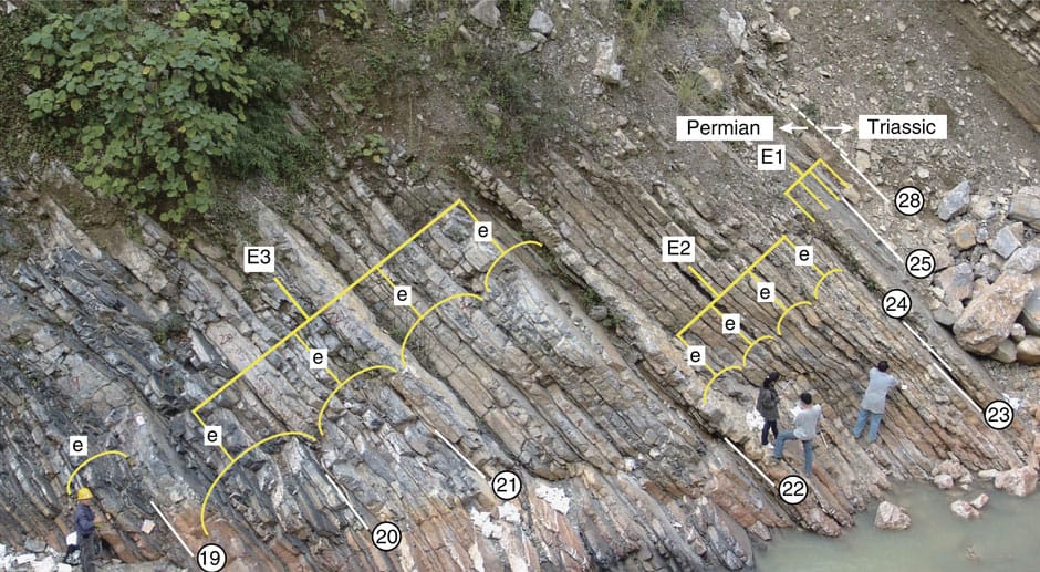
“Rhythmically banded” sections – where older rock formations have Milankovic´ cycles imprinted in the form of colour and particle variations – have been found in almost all parts of the geological record. Shown here is an example of such structures from the Upper Changhsingian Dalong Formation at Shangsi in China, being 252–254 million years old.
Indeed, now that we understand that variations in the Earth’s orbit around the Sun have been such a powerful influence on the record of the past 80 million years of Earth history, it is perhaps not surprising to find that such cycles have affected even earlier times of sedimentary deposition. And yet, all is not straightforward. Although the cycle of glaciations and deglaciations has controlled the oxygen-isotope signal in the deep-sea record over the last 40 million years, the problem is that before then the Earth was ice-free. What then can account for the imprinting of the orbital record on these older cyclic sediments? The probability is that it is the temperature component only, rather than having anything to do with ice volume, particularly at the most sensitive latitudes to incoming solar insolation, which Milankovic´ himself identified as about 65˚N and 65˚S.
And then again, the whole science of astrochronology is based upon the hypothesis that the Earth’s orbital parameters have varied in a uniform and repeatable manner. If these parameters themselves have varied, then some form of correction will need to be devised for any systematic deviations in the astronomically tuned timescale as we delve further and further back into deep time. So next time you find yourself watching George Pal’s version of The Time Machine, with the machine’s endlessly spinning disc, spare a thought for how he correctly, and unawares, saw the future of geology, where time is measured, like his spinning disc, in cycles.