Imaging plays a vital role in diagnosing brain disease and disorders, as well as advancing our understanding of how the human brain works. Existing brain imaging modalities, however, usually require the subject to lie flat and motionless – precluding use in people who cannot remain still or studies of the brain in motion.
To address these limitations, neuroscientists at West Virginia University have developed a wearable, motion-compatible brain positron emission tomography (PET) imager and demonstrated its use in a real-world setting. The device, described in Communications Medicine, could potentially enable previously impossible neuroimaging studies.
“We wanted to create and test a tool that could grant access to imaging the brain – including deep areas – while humans are moving around,” explains senior author Julie Brefczynski-Lewis. “We hope our device could allow the investigation of research questions related to natural upright behaviours, or the study of patients who are normally sedated due to movement issues or challenges in understanding the need to be perfectly still for a scan, which could happen with cognitive impairments or dementias.”
PET scans provide information on neuronal and functional activity by imaging the uptake of radioactive tracers in the brain. But clinical PET systems are extremely sensitive to motion and require supine (lying down) imaging and dedicated scanning rooms. There are neuroimaging techniques that can be used with patients upright and moving – such as functional near-infrared spectroscopy and high-density diffuse optical tomography – but these optical approaches only image the brain surface. Activity in deep brain structures remains unseen.
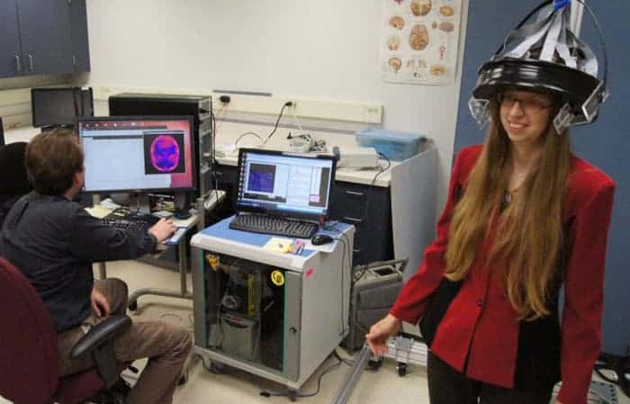
To enable upright and motion-tolerant imaging, Brefczynski-Lewis and colleagues designed the AMPET (ambulatory motion-enabling positron emission tomography), a helmet-like device that moves along with the subject’s head. The imager is made from a ring of 12 lightweight detector modules, each comprising arrays of silicon photomultipliers coupled to pixelated scintillation crystal arrays. The imager ring has a 21 cm field-of-view and a central spatial resolution of 2 mm in the tangential direction and 2.8 mm in the radial direction.
Real-world scenarios
The researchers tested the AMPET device on 11 volunteer patients who were scheduled for a clinical PET scan on the same day. The helmet was positioned the on the participant’s head such that it imaged the top of the brain, comprising the primary motor areas. Although it only weighs 3 kg, the team chose to suspend the helmet from above so that participants would not feel any weight while moving their head.
Patients received a low dose (10–20% of their total prescription) of the metabolic PET tracer 18F-FDG. “We chose a very low dose that was within the daily dose for clinical patients,” says Brefczynski-Lewis. “Some applications may require a slightly higher dose for extra sensitivity, but because the detectors are so close to the head, a full clinical-like dose would not likely be necessary.”
Immediately after tracer injection, each participant underwent AMPET imaging for 6 min while they switched between standing still and walking-in-place every 30 s. Following a 5 min transition, subjects were then scanned for another 5 min while alternating between sitting still and lifting their leg while seated. In this second imaging session, the team moved the AMPET lower around the head for five participants, to image deeper brain structures.
Meeting the goals
The team defined three goals to validate the AMPET prototype: motion artefacts of less than 2 mm; differential activation of cortical regions of interest (ROIs) related to leg movement; and differential activation to walking movements in deep brain structures.
The walking versus standing task allowed the researchers to test for any motion of the imager relative to the head. They observed an average movement-related misalignment of just 1.3 mm. Analysis of task-related activity showed the expected brain image patterns during walking, with activity in ROIs that control leg movements significantly greater than in all other imaged ROIs.
In four participants where activity was measured from deep brain structures (the fifth had incorrect helmet placement), the team observed differential activation in various deep lying structures, including the basal nuclei.
The researchers note that one volunteer had a prosthetic right leg. While performing upright walking, his brain patterns showed greater metabolic activity in the area that represented the intact leg. In contrast, no difference in activity between left and right leg ROIs was measured in the other participants.
Brefczynski-Lewis tells Physics World that patients found the AMPET reasonably comfortable and did not feel its weight on their head or neck. Certain movements, however, were slightly inhibited, especially tilting the head towards the shoulders. “Our engineer collaborators recommended a gyroscope mechanism to enable free movement in all directions,” she says.
As well as validating the prototype, the study also identified upgrades required for the AMPET and similar systems. “The great thing about a real-world study on humans was that it showed us which logistics to optimize,” explains Brefczynski-Lewis. “We are developing a system for good placement and monitoring the alignment of the imager relative to the head, as well as widening the coverage to increase sensitivity, and testing a movement task using a bolus-infusion paradigm.”
Embrace the flaws AI isn’t some sort of all-powerful super brain, but is in fact prone to biases and errors. (Courtesy: iStock/metamorworks)
Artificial intelligence (AI) is rapidly becoming an integral part of our society. In fact, as I write this article, I have access to several large language models, each capable of proofreading and editing my text. While the use of AI can be controversial – who’s to say I really wrote this article? – it may soon be so commonplace that mentioning it will be as redundant as noting the use of a word processor. Just to be clear though, this review is all my own work.
It’s still early days for AI, but it has the potential to impact every aspect of our lives, from politics to education and from healthcare to business. As AI is used more widely, it’s not just computer scientists who need to understand how machines think and come to conclusions. Society as a whole must have a basic appreciation and understanding of how AI works to make informed decisions.
Why Machines Learn, by the award-winning science writer Anil Ananthaswamy, takes the reader on an entertaining journey into the mind of a machine. Ananthaswamy draws inspiration from the subject of his book; much like training a neural network, he uses well-designed examples to build the reader’s understanding step by step.
Whereas AI is a general term that covers human-like qualities such as reasoning and adaptive intelligence, the author’s focus is on the subfield of AI known as “machine learning”, which is all about how we extract knowledge from data. Starting with the fundamentals, Ananthaswamy carefully constructs a comprehensive picture of how machines learn complex relationships.
Anyone who thinks that AI is a modern invention, or that the road to today’s technology has been smooth, will be shocked to learn that the pursuit of a “learning machine” began in the 1940s with McCulloch and Pitts’ model of a biological neuron. Funding for this now billion-dollar industry has sometimes also been meagre. What’s more, the concepts underpinning modern AI have their roots in diverse and unexpected areas, from the idle curiosities of academics to cholera outbreaks and even game shows.
Ananthaswamy’s background in electronics and computer engineering is evident throughout this book, for example in how he introduces several technical and mathematical concepts needed to grasp the power and limitations of machine learning. He begins with the US psychologist Frank Rosenblatt’s development in the late 1950s of the “perceptron” – a basic, single-layer learning algorithm with a binary output (“yes” or “no”). The author then shows how decades of innovation have led to deep neural networks with billions of neurons, such as ChatGPT, capable of giving nuanced and insightful responses.
Unusually for a popular-science book, Why Machines Learn includes quite a lot of mathematics and equations
Unusually for a popular-science book, Why Machines Learn includes quite a lot of mathematics and equations as it explores how vectors, linear algebra, calculus, optimization theory, statistics and probability can be employed to engineer a synthetic brain. Given the complexity of these topics, Ananthaswamy is careful to provide frequent recaps of key concepts so that readers less familiar with these ideas don’t become lost or overwhelmed.
Fortunately, the author has the uncanny ability to answer questions with simple and illuminating examples just as they arise in the reader’s mind. Although this might seem to diminish some of the magic, it’s inspiring to see how such a powerful system can be constructed from deceptively simple components.
Gaming the system
For topics such as probability, this pedagogical approach is essential for anyone without a strong background in mathematics. For instance, the infamous Monty Hall problem is so counterintuitive that even some of the world’s most renowned mathematicians struggled to accept its solution. Indeed, as Ananthaswamy notes, Paul Erdős – one of the most prolific mathematicians of the 20th century – “reacted as if he’d been stung by a bee” when confronted with the answer.
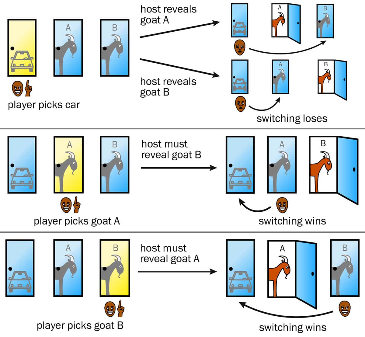
Intelligence test Based on the US game show Let’s Make a Deal, the Monty Hall problem involves three doors, behind which are two goats and a car. The contestant on the show picks a door, without seeing what’s behind it, before the host opens one of the other doors to reveal a goat: the contestant then has to decide whether to swap to the other, unopened door. The logic behind the problem is a cornerstone of machine learning. (Courtesy: IOP Publishing)
The dilemma is based on the classic US TV game show Let’s Make a Deal, hosted by Hall, in which you, the contestant, have a choice of three doors. Behind one is a brand-new sports car, while the other two doors conceal goats. After you pick a door (but don’t get to see what’s behind it) the host opens one of the other two doors to reveal a goat. The host then offers you the chance to switch your choice to the remaining, unopened door.
To maximize your chances of winning the car, you should always switch. It’s counter-intuitive and controversial. Surely, if you’ve got two doors to pick from, then the odds of getting the car must be 50–50? In other words, why would you bother switching if there’s a car behind one door and a goat behind the other? The book goes on to explain how the logic behind this decision is a cornerstone of machine learning; bypassing human intuition, which is often flawed.
Ananthaswamy shows that machine learning is a powerful method of analysis. He first demonstrates how data can be represented in an abstract, high-dimensional space, before explaining how collapsing the number of dimensions allows patterns in the data to be found. With the assistance of some elegant linear algebra, this process can be engineered so that the data is categorized most effectively; highlighting strong correlations, which leads to more reliable performance.
Cautious embrace
In our data-driven world, this remarkable capability of AI is something that should be embraced. However, like any data-analysis method, machine learning is prone to biases and errors. Why Machines Learn gives the reader an awareness and understanding of these shortcomings, allowing AI to be used more effectively.
This is particularly important as AI becomes mainstream. It’s common for people to mistakenly believe that it’s some all-powerful super brain, capable of completing any task with ease. This misconception can lead to the misuse of AI or the unfair perception of AI as overrated when it falls short of this unrealistic standard. Ananthaswamy gives his readers an appreciation of how machine learning works and, hence, how to use it appropriately, which may help combat the abuse of AI.
It’s evident that machines are far from achieving human-like intelligence
By exploring the fundamental principles of machine learning in such detail, it’s evident that machines are far from achieving human-like intelligence. While the secrets of the human brain remain elusive, Why Machines Learn demystifies the underlying mechanisms behind machine learning, which may possibly lead to a better understanding of the learning process itself and the development of improved AI.
This inevitably requires the reader to confront advanced and counterintuitive concepts in various branches of mathematics and logic, from collapsing dimensions to mind-bending games of chance. For those who invest the time and effort, they will reap the rewards that come from understanding a technology with the potential to revolutionize many aspects of our lives.
The synchronized flashing of fireflies in summertime evokes feelings of marvel and magic towards nature. How do they do it without a choreographer running the show?
For some physicists, though, these natural fireworks also raise other questions. If the fireflies were quantum, they wonder, would they synchronize their flashing routines faster or slower than their classical counterparts?
Questions of this nature – about how quantum systems synchronize, the energetic costs they pay to do so, and how long it takes them to fall into lockstep – have long bedevilled physicists. Now a team of theorists in the US has begun to come up with answers. Writing in Physical Review Letters, Maxwell Aifer and Sebastian Deffner of the University of Maryland Baltimore County (UMBC), together with Juzar Thingna of the University of Massachusetts, Lowell (UMass Lowell), present a new take on the energetic cost and time required to synchronize quantum systems. Among other findings, they conclude that quantum systems can synchronize in scenarios where such behaviour would be impossible classically.
How quantum springs synchronize
Studies of synchronization go back to the 1600s, when Christiaan Huygens documented that pendulums placed on a table eventually sway in unison. Huygens called this the “sympathy of pendulums”.
This apparent sympathy between systems – chirping crickets, flashing fireflies, the harmonious firing of pacemaker cells in our hearts – turns out to be ubiquitous in nature. And while it may look like magic, it ultimately stems from information exchanged between individual systems via communication pathways (such as the table in the case of Huygens’ pendulums) available in the shared environment.
“At its core, synchronization is about balance of forces,” Thingna says.
To understand how that balance works, imagine you have a bunch of systems moving in circles of different sizes. The radius of the circle corresponds to the amount of energy in that system.
At first, the systems may all be moving at different paces: some faster, others slower. To synchronize, the circles must interact in such a way that gradually, the radius of all the circles and the pace of the systems becomes the same – meaning that bigger circles must “leak” energy and smaller circles gain it.
But synchronization is impressive only when it is resilient and robust. This means that if there are small disturbances – for example, if one of the systems is kicked out of its circle – the disturbed system should return to the radius and pace of the others.
This picture works for classical systems, but synchronization in the quantum regime is more complex. “The challenge lies in translating the classical concept of synchronization to the quantum world where trajectories are ill-defined concepts due to Heisenberg’s uncertainty principle,” explains Christopher Wächtler, a quantum physicist at the University of California, Berkeley, US who was not involved in this work.
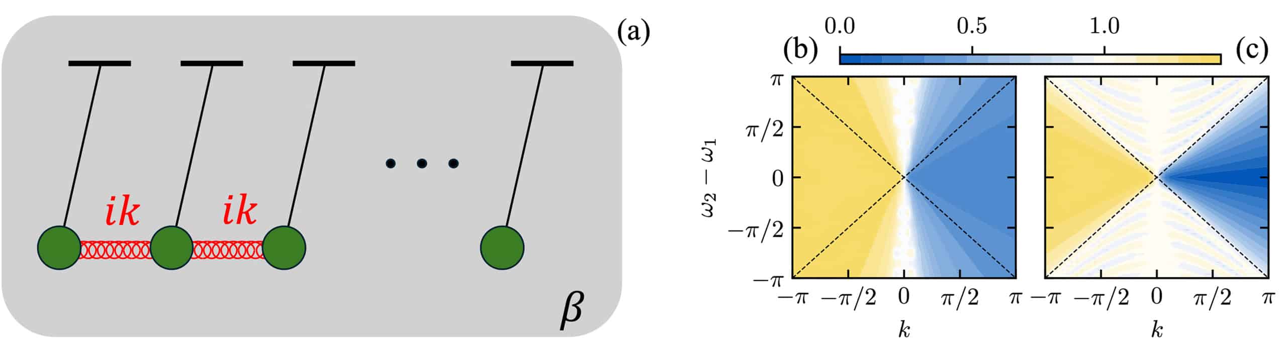
Synchronization: a) A bunch of pendulums (oscillators) interacting with each other via anti-Hermitian coupling of strength k and with a common environment at a fixed temperature. The synergetic effects of non-Hermitian coupling and the thermal reservoir help the system collectively synchronize. b) and c) Synchronization measured as a function of the non-Hermitian interaction strength k and the frequency difference ω1-ω2 for a minimal two oscillator quantum system (N=2) for quantum (b) and classical (c) evolution. White region indicates the absence of synchronization, whereas the coloured (blue or yellow) regions indicate that the system synchronizes. For the classical system, the synchronizing regime is restricted within the dashed lines, while the quantum system is robust and synchronizes in regimes where it is impossible for the classical system to do so.(Courtesy: Juzar Thingna)
Taking inspiration from an experimental setup, the UMBC-UMass Lowell team created a model based on quantum oscillators or springs (a well-known quantum system) that interact with each other via a biased channel – an anti-Hermitian coupling in which one oscillator is favoured more than the other. This biased channel controls the flow of energy in and out of the individual springs. The oscillators also leak information by “talking” to a common thermal environment at a given temperature.
Thanks to this combination of a common thermal environment and a biased inter-system communication channel, the team was able to balance the information flow (that is, the communication between the oscillators and communication with the environment) and synchronize quantum systems in a way similar to how classical systems are synchronized.
The economics of sympathy
This approach is unusual because quantum synchronization research typically explores the quantum systems in their synchronized state after they have been coupled for a long time. In this case, however, the researchers focus on the time before the steady state has been reached, “which in my opinion is an important question to ask,” says Christoph Bruder, a physicist at the University of Basel, Switzerland who was not involved in the study.
To estimate the time it takes to synchronize, the UMBC-UMass Lowell researchers use quantum speed limits, which are a mathematical way of deriving the maximum time it takes a system to go from an initial state to a desired final state. They find that quantum oscillators synchronize the fastest when the conversations between oscillators do not leak – that is, the strength of the interaction between the oscillators outweighs the interaction with the environment.
The team also used ideas from quantum thermodynamics to identify a lower bound on the energetic cost of synchronization. This bound depends on the biased way in which the oscillators talk to each other.
But there is no free lunch.
While synchronizing a small number of quantum systems is energetically more efficient than doing the same for a classical counterpart, the researchers report that this is not scalable. When there are many systems, classical systems are more energy efficient than quantum ones. However, the researchers found that a model system does exhibit quantum synchronization for a wider range of interaction strengths than is the case for classical oscillators, making synchronization in the quantum regime more resilient and robust.
Though the work is still theoretical at this point, Wachtler says that a minimal version of the team’s model could be “effectively implemented in a lab”. The team is keen to explore this further. “For us, this is the first stepping-stone towards this goal of how to make synchronization more practical,” Thingna says.
A prototype argon detector belonging to the Deep Underground Neutrino Experiment (DUNE) in the US has recorded its first accelerator-produced neutrinos. The detector, located at Fermilab near Chicago, was installed in February in the path of a neutrino beamline. After what Fermilab physicist Louise Suter calls a “truly momentous milestone”, the prototype device will now be used to study the interactions between antineutrinos and argon.
DUNE is part of the $1.5bn Long-Baseline Neutrino Facility (LBNF), which is designed to study the properties of neutrinos in unprecedented detail and examine the differences in behaviour between neutrinos and antineutrinos. Construction of LBNF/DUNE began in 2017 at the Sanford Underground Research Facility in South Dakota, which lies some 1300km to the west of Fermilab. When complete, DUNE will measure the neutrinos generated by Fermilab’s accelerator complex.
Earlier this year excavation work was complete on the two huge underground spaces that will be home to DUNE. Lying 1.6km below ground in a former gold mine, the spaces are some 150 m long and seven storeys tall and will house DUNE’s four neutrino detector tanks, each filled with 17 000 tonnes of liquid argon. DUNE will also feature a near-detector complex at Fermilab that will be used to analyze the intense neutrino beam from just 600 m away.
The “2×2 prototype” detector, so-called because it has four modules arranged in a square, record particle tracks with liquid argon time-projection chambers to reconstruct a 3D picture of the neutrino interaction.
“It is fantastic to see this validation of the hard work put into designing, building and installing the detector,” says Suter, who co-ordinated installation of the modules.
It is hoped that the DUNE detectors will become operational by the end of 2028.
Any good sailor knows that the right choice of knot can mean the difference between life and death. Whether it hoists the sails or secures the anchor, a rope is only as good as the knot that’s tied in it. The same is true, on a much smaller scale, for many of the molecules that keep us alive.
Proteins are essential building blocks for all living things, and these long chains of amino acids form complex 3D shapes that allow molecules to fit together. For a long time, it was thought that while proteins can be highly tangled, they could not form knots under normal conditions, as this would prevent the proteins from being able to fold. But in the 1970s researchers found many topologically knotted proteins, in which their native structures are arranged in the form of an open knot.
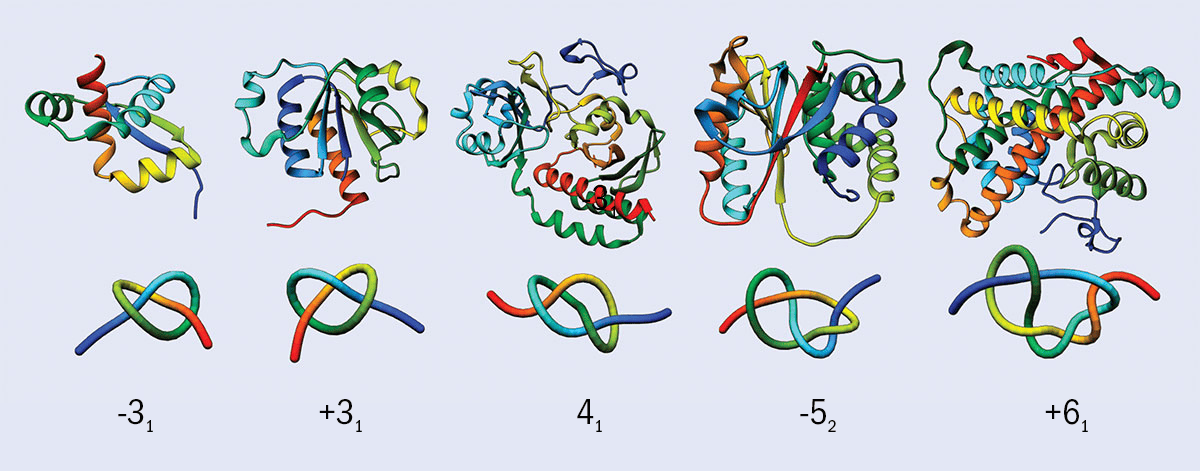
As it happens, despite proteins (and even DNA) having “open” curves, knots can still form and affect their function. Indeed, they comprise about 1% of proteins in the Protein Data Bank. Unlike a rope or string, each protein of this type has a characteristic knot (figure 1). The largest group of knotted proteins is the SPOUT family of enzymes (which make up the second largest of seven structurally distinct groups of methyltransferases enzymes), all but one of which are knotted in a “trefoil” of three overlapping rings.
Some proteins form well-defined knotted structures, as shown above, where the lower image shows a simplified view of each molecule. The number below each image indicates the number of times the protein crosses itself and the + and – indicate that they are mirror images. The –31 and +31 for example are mirror image instances of the “trefoil” knot. Proteins form “open knots” because their two ends don’t join up. However, it is often still possible to define a knotted structure in the molecule.
This discovery raised many questions, such as how and why these knots form, what is the mechanism of their folding, and what role this might play on a functional level. There is some evidence that knotted proteins are more resistant to extreme temperatures, but scientists still do not know how abundant knots are in molecular structures or exactly how knotting affects their biological function.
The trouble is that when we try to apply what we know about knots to questions in biology and soft matter, we come up against a mathematical problem that’s been confounding scientists for over a century.
A tangled history
The origins of modern knot theory are often traced back to a famous experiment that was performed more than 150 years ago – not with ropes or string, but with smoke.
In 1867 Peter Guthrie Tait invited his friend and fellow physicist William Thomson (later Lord Kelvin) to travel from Glasgow to Edinburgh to witness a demonstration where he generated pairs of smoke rings. To Kelvin’s surprise, these rings were remarkably stable, travelling across the room and even bouncing off each other as if they were made of rubber. A smoke ring is a “vortex ring” in which the aerosols and particulates are rotating in small concentric circles, and this motion gives the ring its stability.
At the time, it was widely believed that the universe was pervaded by a space-filling substance dubbed “aether”, through which gravitational and electromagnetic radiation propagated. Kelvin reasoned that atoms might be made from stable vortices, like smoke rings, in this aether. He further argued that knots tied in aether vortex rings could account for the different chemical elements.
The vortex theory of atoms was incorrect, but knot theory continues to this day as a branch of mathematics
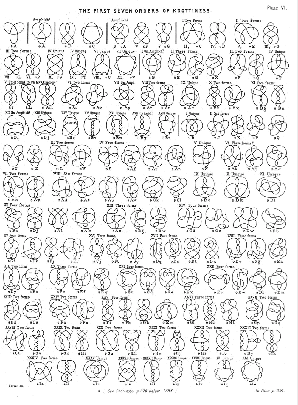
Tait was intrigued by Kelvin’s theory. Over a period of 25 years, and with the help of the Church of England minister Thomas Kirkman, American mathematician Charles Little and James Clerk Maxwell, Tait produced a table of 251 knots with up to 10 crossings (figure 2). The vortex theory of atoms was incorrect, but knot theory continues to this day as a branch of mathematics.
2 Order and disorder
(Taken from “On knots part II” published in 1884. Image courtesy of the University of St Andrews Library, ID sfQC3-T2-Vol-1-6)
Peter Guthrie Tait and other early knot theorists spent years compiling a comprehensive list of knots. The above image is extracted from their table of knots up to seven crossings – “the first seven orders of knottiness”.
Spot a knot
For Tait and his fellow theorists, the classification of knots was painstaking work. Every time a new knot was proposed, they had to check that it was unique using drawings and geometric intuition. Tait himself wrote that “though I have grouped together many widely different but equivalent forms, I cannot be absolutely certain that all those groups are essentially different from one another”. Indeed, in 1974 Kenneth Perko showed that two entries in the original table are actually the same knot – these are now known as the “Perko pair” (Proc. Amer. Math. Soc.45 262).
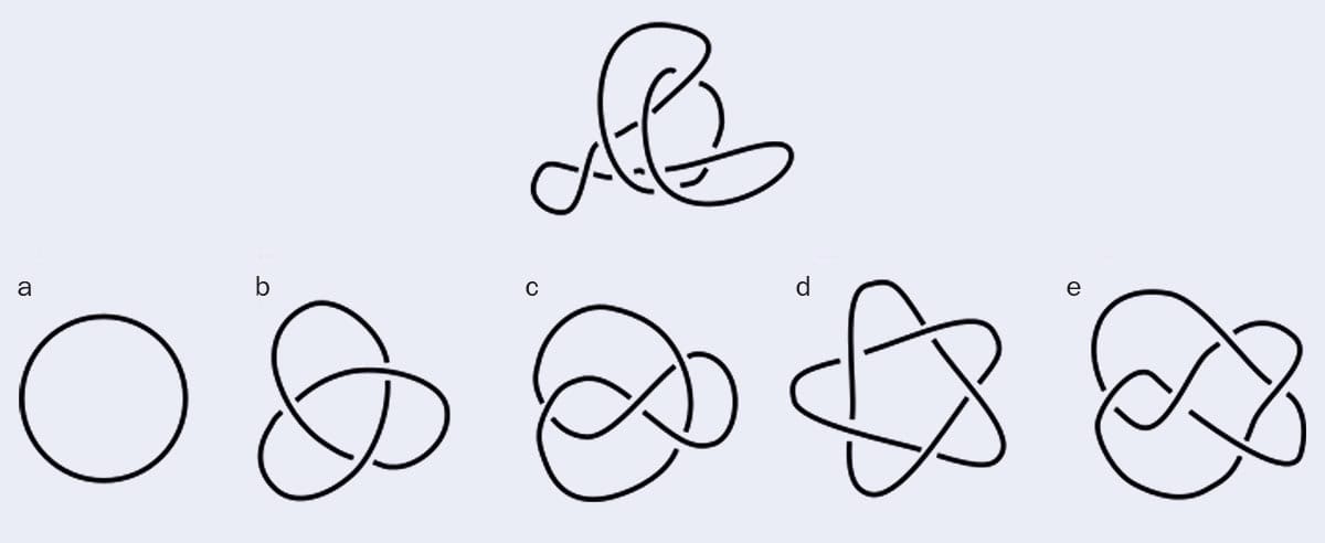
If you need any more convincing, my student Djordje Mihajlovic has developed an online game called “Spot a Knot” where the goal is to spot equivalent knots from pictures (figure 3). Even after years of researching knots, I often get it wrong. To earn a spot in the table, a knot must have a unique topology, meaning that it cannot be deformed into any other known knot without being broken. As the Perko pair and Mihajlovic’s game show, proving that two knots are different is easier said than done. Remember that topology studies the properties of spaces that do not change if they are deformed smoothly; to a topologist, a mug is equivalent to a doughnut because one can be massaged into the other without losing the inner hole.
3 Brain teaser
(Courtesy: Djordje Mihajlovic)
To illustrate the difficulty of identifying knots, Djordje Mihajlovic – a PhD student at the University of Edinburgh – developed an online game called “Spot a Knot”. One question is reproduced above. Does the top image correspond to a, b, c, d or e?
As scientists learned more about the structure of the atom, the vortex atom model was gradually abandoned. A final blow came in 1913 when Henry Moseley showed that chemical elements are differentiated not by their topology but by the number of protons in the nucleus.
In knot theory, quantities that describe the properties of knots are called “invariants”. The dream of knot theorists is to find a quantity like the proton number that can classify any knot based on its topology. Such a “complete invariant” would yield a unique value for every unique knot, and wouldn’t change if the knot were smoothly deformed.
A recipe for such a topological invariant could be something like this: “Walk along the knot and label each of the n crossings with numbers 1, 2, 3, …, 2n (you will traverse the knot twice). If the label is even and the line is an overcrossing, then change the sign of the label to minus (figure 4). At the end, each crossing will be labelled by a pair of integers, one even and one odd. The series of even integers is a code for the knot.” This recipe is called the Dowker–Thistlethwaite code, first proposed in 1983 (Topology and its Applications16 19) (figure 5).
The Dowker–Thistlethwaite code can classify many simple knots, but like every other method that’s been proposed, it isn’t a complete invariant. The first knot invariant was proposed in 1928 by James W Alexander and called the Alexander polynomial. Since then, many others have been developed, but for each one, a case has been found where it fails to make a unique classification.
Taking a walk
The Alexander polynomial belongs to the family of so-called “algebraic invariants”. It is computed by constructing a matrix with as many rows and columns as there are crossings in the knot, and taking its determinant. Algebraic invariants are constructed from a 2D projection of the knot. This is a bit like a shadow, but one where we can discern which part of the loop is on top each time it crosses itself.
Soft-matter physicists like myself, however, want to classify the knots in molecules like proteins and DNA, which are 3D and constantly jostled by thermal energy. Reducing these molecules to 2D projections erases spatial features that may be crucial to their function.
An attractive alternative for characterizing molecules is “geometric invariants”. These are calculated by traversing the knot in 3D and computing some geometric property, such as the curvature, along the route.
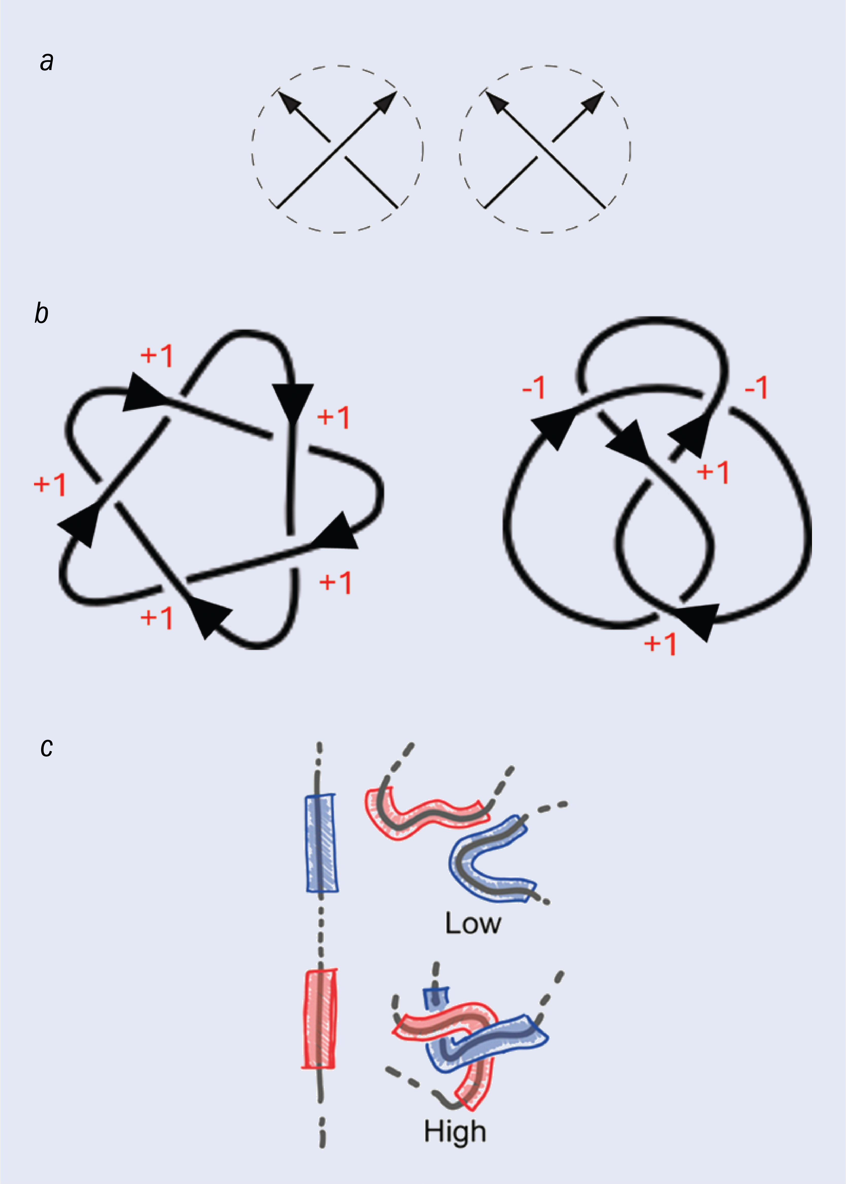
One such invariant that I am fond of is the “writhe”, which was introduced by Tait. Writhe can be measured on a 2D projection by counting the “over” and “under” crossings and subtracting one from the other (figure 4b).
One way to tell the difference between knots is to measure the “writhe”, which quantifies the amount of twisting. (a) Each time the knot crosses itself, the crossing can be characterized as either an overcrossing (left) or an undercrossing (right). The writhe is calculated by subtracting the number of undercrossings from the number of overcrossings.
(b) How the writhe is calculated for two knots – the cinquefoil knot (left), which has a writhe of +5, and the figure-eight knot (right), which has a writhe of 0.
(c) The writhe can also be calculated as a geometric quantity on a 3D molecular knot such as a protein. The geometric writhe can be calculated over the entire knot or as a local quantity between short, adjacent strands. A high value of the “local writhe” indicates that the strands are entangled with each other. Davide Michieletto and colleagues showed that a neural network trained on the local writhe characterizes knot topology with high accuracy.
However, writhe can also be computed as a geometric quantity. Imagine walking along a 3D knot, such as a protein, and at each step writing down an estimate of the writhe by counting the crossings you can see. At the end of your journey, the average of these numbers will yield the true value of the writhe. Unfortunately, writhe isn’t a complete invariant. In fact, like its algebraic counterparts, no geometric invariant has ever been proved to uniquely classify all knots.
In 2021 Google DeepMind’s AlphaFold artificial-intelligence programme solved a problem that had been evading scientists for decades – how to predict a protein’s structure from its amino acid sequence (Nature596 583). The function of proteins depends on their 3D structure, so AlphaFold is a powerful tool for drug discovery and the study of disease.
The question we asked ourselves was: could AI do the same for the knot invariant problem?
Wriggle and writhe
Using AI to classify knots has been explored by previous researchers, most recently by Olafs Vandans and colleagues of the City University of Hong Kong in 2020 (Phys. Rev. E 101 022502) and Anna Braghetto of the University of Padova and team in 2023 (Macromolecules56 2899). In those studies, they treated the different knots like strings of beads and trained a neural network to identify them by giving it the Cartesian coordinates and, in the latter case, the vector, distance and angles between the beads.
5 Encoding knots
(Public domain)
The Dowker–Thistlethwaite notation is a knot-invariant first proposed in 1983. This method assigns a sequence of integers to a knot by traversing it twice and assigning a number to each crossing, as shown in the image. The final sequence characterizes the knot.
These researchers achieved high accuracies, but only for the five simplest knots. We wanted to extend this to much more complicated topologies, while also simplifying the neural network architecture and using a smaller training dataset.
To do this we took inspiration from nature. In our bodies, knots in DNA are untangled by specialist enzymes called topoisomerases. These enzymes cut and reattach DNA strands and they can effectively smooth out knots despite being about a thousand times smaller than a DNA molecule.
We hypothesized that the topoisomerases can sense some local geometric property that allows them to locate the most tightly knotted part of the DNA molecule. We tried to do this ourselves using various quantities including the density and the curvature. In the end our results led back to the beginning – to Tait and his geometric writhe.
We decided that giving our AI the local writhe would give it the best chance to successfully identify complex knots
As well as calculating writhe over an entire knot, we can also measure it as a local quantity that tells us how much segment x is entangled with nearby segment y (figure 4c). We found that local writhe is a remarkably effective way to locate knotted segments in long, looping molecules (ACS Polymers Au2 341). Based on this result, we decided that giving our AI the local writhe would give it the best chance to successfully identify complex knots.
Armed with our theory, we began building a neural network to test it. To start, we generated a training dataset by simulating the thermal motion of the five simplest knots, extracting tens of thousands of conformations (figure 6a).
We then trained two neural networks: one using the Cartesian coordinates of the knots and one using the local writhe. In each case, we supervised the AI, and used a subset of our training dataset to tell the neural networks what type each of the knots was. To test our method we asked the neural networks to classify conformations of these simple knots that they hadn’t seen before.
When the AI was trained on the Cartesian coordinates on a simple neural network, it made a correct categorization only four times out of five, similar to what Vandans and Bragetto found. This is probably better than the score most of us would get in the Spot a Knot game, but it’s still far from perfect.
However, when the neural network was trained on the local writhe, the difference was staggering: it could correctly classify the knots with more than 99.9% accuracy.
Tougher challenges
Though I was surprised by this result, the identification of the five simplest knots is relatively trivial, and can be achieved using existing invariants (or an extremely eagle-eyed Spot a Knot player).
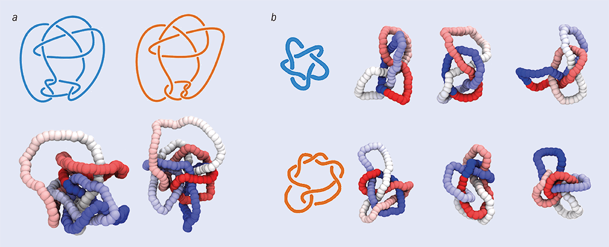
We decided to give the neural network a much trickier challenge. This time it would only have to classify three knots rather than five, but we had chosen them carefully: the Conway knot, the Kinoshita–Terasaka (KT) knot and the unknot – the simplest of all knots. The first two have 11 crossings, and are “mutants” of each other because they are identical except in one region where the knot is “flipped”. They share many knot invariants, and they also share some invariants with the unknot.
6 Spot the difference
(a) CC BY 3.0 Davide Michieletto et al.Soft Matter20 71; (b) Courtesy: Davide Michieletto
A complete knot invariant shouldn’t change when a knot is smoothly deformed, but should return a different result for topologically distinct structures. Do the two pictures in a show the same knot? It’s often difficult for human intuition to tell knots apart. In fact, the two pictures show two slightly different structures – the Conway and Kinoshita–Teresaka knots. Because it’s difficult to tell them apart, these two knots can be used to test a knot-characterization neural network.
The images in b show different configurations of two knots – the 51, or cinquefoil knot (above) and the 72 knot (below). In Davide Michieletto and colleagues’ work on neural networks, the cinquefoil was part of the first training dataset and the 72 was included in the larger dataset.
What we discovered is that the Conway and KT knots were indistinguishable for a neural network trained on Cartesian coordinates but they could be identified 99.9% of the time by the neural network trained on the local writhe.
The final test was to apply this training to a much larger pool of knots. We ran simulations of 250 types of knots, with up to 10 crossings (figure 6b). When the neural network was trained with the Cartesian coordinates it made a correct classification only one time out of five. By contrast, our best local-writhe-trained neural network could classify all 250 knots in a matter of seconds with 95% accuracy, much better than any other algorithm or single topological invariant (Soft Matter20 71).
A final twist
Without knowing anything about knots or knot theory, our neural network had taught itself to do something that has long evaded human intuition. In fact, we are still working to open the “black box” and understand what exactly it discovered.
We have found that to distinguish the five simplest knots, the neural network takes every set of pairs of points on the knot and multiplies the writhe at the two points together. What’s intriguing is that this quantity is equivalent to an existing invariant called the “Vassiliev invariant of order two”.
Vassiliev invariants are computed by multiplying pairs, triplets, quadruplets, up to n-tuples of the local writhe matrix. Incidentally, the Vassiliev invariant of order 2 is also the coefficient of the quadratic term of the Conway polynomial, the algebraic invariant we saw earlier. It’s been proposed, though never proved, that the complete set of Vassiliev invariants, which can be computed as an integral, is the long-searched-for complete invariant.
We were excited to find that as it’s presented with more complex knots, the neural network adapts by computing Vassiliev invariants of higher order
We were therefore excited to find that as it’s presented with more complex knots, the neural network adapts by computing Vassiliev invariants of higher order. For instance, to uniquely classify the first five knots, the neural network requires only the degree two Vassiliev invariant. But for the 250-knot dataset, it may compute the Vassiliev invariants up to order three or four.
Geometric and algebraic invariants are computed using very different mathematics, so it’s exciting that AI can discover connections between them, and this brings us a step closer to discovering a complete invariant.
Knotting else matters
In only three years, AlphaFold has generated millions of proteins, most of which have yet to be fully studied. In 2023 a group led by Joanna Sulkowska of the University of Warsaw predicted that up to 2% of human proteins generated by AlphaFold are knotted, with the most complex knot found having six crossings (Protein Sci. 32 e4631). The year before, Peter Virnau of the Johannes Gutenberg University Mainz discovered a protein knot with seven crossings in the AlphaFold2 dataset (Protein Sci. 31 e4380). This protein has never been observed experimentally, so it’s possible that even more complex knots are out there.
Knots don’t crop up only in biology; knotted topologies have also been found to influence the thermodynamic and material properties of ice and hydrogels; meaning that in the future, we may use topology to design new materials. We need powerful methods to identify the structural fingerprints of knots in molecules and materials and we hope that our findings will inform this search. Knotting really does matter.
In 2004 three researchers in Canada used their university’s computing cluster to extend the table of knots, first compiled by Tait, up to 19 crossings, identifying more than six billion unique structures (Journal of Knot Theory and Its Ramifications13 57). Having taken 25 years to create his list, Tait would probably have been shocked to learn that a century later, a machine would be able to extend his work by more than five orders of magnitude, in just a few days.
The biggest outstanding challenge in knot theory remains the search for the elusive complete invariant. Now that we are enabled by AI, the next step forward might take us equally by surprise.
When former physicist James Gillies sat down for dinner in 2009 with actors Tom Hanks and Ayelet Zurer, joined by legendary director Ron Howard, he could scarcely believe the turn of events. Gillies was the head of communications at CERN, and the Hollywood trio were in town for the launch of Angels & Demons – the blockbuster film partly set at CERN with antimatter central to its plot, based on the Dan Brown novel.
With CERN turning 70 this year, Gillies joins the Physics World Stories podcast to reflect on how his team handled unprecedented global interest in the Large Hadron Collider (LHC) and the hunt for the Higgs boson. Alongside the highs, the CERN comms team also had to deal with the lows. Not least, the electrical fault that put the LHC out of action for 18 months shortly after its switch-on. Or figuring out a way to engage with the conspiracy theory that particle collisions in the LHC would somehow destroy the Earth.
Spoiler alert: the planet survived. And the Higgs boson discovery was announced in that famous 2012 seminar, which saw tears drop from the eyes of Peter Higgs – the British theorist who had predicted the particle in 1964. Our other guest on the podcast, Achintya Rao, describes how excitement among CERN scientists became increasingly palpable in the days leading to the announcement. Rao was working in the comms team within CMS, one of the two LHC detectors searching independently for the Higgs.
Could particle physics ever capture the public imagination in the same way again?
Photons in arrays of nanometre-sized structures exhibit more complex behaviour than electrons in conventional solid-state materials. Though the two systems are sometimes treated as analogous, scientists at the University of Twente in the Netherlands discovered variations in the shape of the photons’ orbitals. These variations, they say, could be exploited when designing advanced optical devices for quantum circuits and nanosensors.
In solid-state materials, electrons are largely confined to regions of space around atomic nuclei known as orbitals. Additional electrons stack up in these orbitals in bands of increasing energy, and the scientists expected to find similar behaviour in photons. “It has been known for some time that photonic materials are similar to standard electronic matter in many ways and can be described using energy bands and orbitals, too,” says Marek Kozon, a theorist and mathematician who participated in the study as part of his PhD in the Complex Photonic Systems (COPS) lab at Twente.
“Similar” does not mean “same”, however. “We have now discovered that orbitals in which photons are confined are significantly more varied in shape than electronic orbitals,” Kozon says. This is important, he says, because the shape of electronic orbitals influences materials’ chemical properties – something that is apparent in the Periodic Table of the Elements, which groups elements with similar orbital structures together. Additional variations in the shape of photonic orbitals could also create properties not achievable in electronic materials.
Boring electrons, exciting photons
The comparatively “boring” behaviour of electrons stems from the fact that they always orbit the nucleus in regions with sphere-like shapes, explains Kozon, who is now at the single-photon detector company Pixel Photonics in Germany. Photonic materials, in contrast, can be designed with much more freedom.
In the latest work, the Twente researchers used numerical computations to study how photons behave when they are confined in a three-dimensional nanostructure known as an inverse woodpile superlattice. This superlattice is a photonic crystal that contains periodic defects with a radius that differs from that of the pores in the underlying structure. The researchers adopted this design for two reasons, Kozon explains. The first is that photonic states inside the defects are insulated from their environment, making them easier to study. The second is that 3D inverse woodpile superlattices are relevant to experiments being carried out by colleagues in the COPS lab.
The team’s original motivation, Kozon continues, was to better understand how light is confined in these structures. “The study turned out be significantly more complicated than we expected,” he says. “We produced several terabytes of data and developed new analysis methods, including scaling and machine learning, to evaluate the sheer amount the information we had gathered. We then investigated in more detail the superlattice parameters that the analysis flagged up as the most interesting.”
Applying the scaling techniques, for example, created an unexpected issue. While scaling theories usually work well for very large systems, which in this case would mean very large periodicities (or lattice constant), Kozon notes that “our system is precisely the opposite because it has a small periodicity. We were thus not able to calculate how light behaves in it.”
Optimally confining light
The team solved this problem by developing a unique clustering method that uses unsupervised machine learning to analyse the data. Thanks to these analyses, the researchers now know which types of structures can optimally confine light in an inverse woodpile superlattice. Conversely, they can identify any deviations from these ideal structures by comparing experimental observations with their – now vast – database.
And that is not all: the team also analysed where energy is concentrated in the photonic crystal, making it possible to determine which parameters allow the greatest concentration of energy in a small volume of the structure. “This is extremely important for so-called cavity-quantum-electrodynamics (QED) applications in which we force light to interact with matter and, for example, to control the emission of light sources or even create exotic states of mixed light and matter,” Kozon tells Physics World. “This finding could help advance applications in efficient lighting, quantum computing or sensitive photonic sensors.”
The Twente researchers are now fabricating real 3D superlattices thanks to the knowledge they have gained. They report their present work in Physical Review B.
An ocean’s worth of liquid water could be trapped within the cracks of fractured igneous rocks deep within the Martian crust – according to a trio of researchers in the US. They have analysed seismic data gathered by NASA’s InSight Lander and their results could explain the fate of some of the liquid water that is believed to have existed on the Martian surface in the distant past.
Mars’ surface carries many traces of its watery past including remnants of river channels, deltas, and lake deposits. As a result, scientists are confident that lakes, rivers, and oceans of liquid water were once common on the Red Planet in the distant past.
Evidence also suggests that about 3–4 billion years ago, Mars’ atmosphere was gradually lost to space, and its surface dried up. While some water remains locked away in Martian ice caps, most of it would have either escaped into space with the rest of the atmosphere, or filtered down into porous rocks in the crust, where it could remain to this day. So far, scientists are uncertain as to how much of this water is held within the crust, and how deeply it could be sequestered.
Seismic insight
This latest research was done by Michael Manga at the University of California Berkeley along with Vashan Wright and Matthias Morzfeld at the University of California San Diego. The trio searched for buried water by analysing data collected by the InSight Lander, which probed the Martian interior in 2018–2022. To gather information about the planet’s crust, InSight’s SEIS instrument detected the seismic waves reverberate throughout the planet, originating from sources including Marsquakes and meteor impacts.
As they travel through the Martian interior, these waves change speed and direction at boundaries between different materials in the crust. This means that when measured by SEIS, seismic waves originating from the same source can be detected at different times, depending on the paths they took to reach the probe.
“The speed at which seismic waves travel through rocks of different densities depend on their composition, pore space, and what fills the pore space – either gas, water, or ice,” Manga explains. By analysing the differing arrival times of seismic waves reaching the probe from the same sources, researchers can gather useful information about the composition of the planet’s interior.
To interpret InSight’s seismic data, Manga and colleagues combined its measurements with the latest rock physics models and probabilistic analysis. They were able to identify the combinations of rock composition, water saturation, porosity, and pore shape within the Martian crust that could best explain InSight’s measurements.
Large reservoir
“We identified a large reservoir of liquid water,” Manga describes. “The observations on Mars are best explained by having cracks in the mid-crust that are filled with liquid water.”
The researchers reckon that this reservoir is sequestered between about 11.5–20 km beneath the surface and contains enough water to cover the Martian surface in a liquid ocean between 1–2 km deep. This section of the crust is believed to comprise fractured igneous rock, formed through the cooling and solidification of magma.
The team hopes that their results could provide fresh insights into the fate of the liquid water that once dominated Mars’ surface. “Understanding the water cycle and how much water is present is critical for understanding the evolution of Mars’ climate, surface, and interior,” Manga says.
The team’s discoveries could help identify potentially habitable environments hidden deep within the Martian crust where microbial communities could thrive today, or in the past.
“On Earth, we see life deep underground,” Manga explains. “This does not necessarily mean there is also life on Mars, but at least there are environments that could possibly be habitable.”
Small leaks of radioactive material can be the death knell for large scientific facilities. It’s happened twice already. Following releases of non-hazardous amounts of tritium, the Brookhaven National Laboratory (BNL) was forced to shut its High Flux Beam Reactor (HFBR) in 1997, while the Lawrence Berkeley National Laboratory (LBNL) had to close its National Tritium Labeling Facility in 2001.
Fortunately, things don’t always turn out badly. Consider the Fermi National Accelerator Laboratory (Fermilab) near Chicago, which has for many decades been America’s premier high-energy physics research facility. In 2005, an experiment there also leaked tritium, but the way the lab handled the situation meant that nothing had to close. Thanks to a grant from the National Science Foundation, I’ve been trying to find out why such successes happen.
Running on grace
Fermilab, which opened in 1971, has had a hugely successful history. But its relationship with the local community got off to a shaky start. In 1967, to acquire land for the lab, the State of Illinois used a US legal manoeuvre called “eminent domain” to displace homeowners, angering neighbours. More trouble came in 1988, when the US Department of Energy (DOE) considered Fermilab as a possible site for the 87 km circumference Superconducting Supercollider (SSC), which would require acquiring more land.
Some locals formed a protest group called CATCH (Citizens Against The Collider Here). It was an aggressive organization whose members accused Illinois officials of being “secretive, arrogant, and insensitive”, and of wanting to saddle the area with radiation, traffic and lower property values. While Illinois officials were making the bid to host the SSC, the lab was the focus of protests. The controversy ended when the DOE chose to site the machine in Waxahachie, Texas. (The SSC was cancelled in 1993, incomplete.)
Aware of the local anger, Fermilab decided to revamp its public relations. In 1989, it replaced its Office of Public Information with a “Department of Public Affairs” reporting to the lab director. Judy Jackson, who became the department’s head, sought professional consultants, and organized a diverse group of community members with different backgrounds, including a CATCH founder, to examine Fermilab’s community engagement practices.
Brookhaven’s closure of the HFBR in 1997 was a wake-up call for US labs, including Fermilab itself. Aware that the reactor had been shut by a cocktail of politics, activism and media scare stories, the DOE organized a “Lessons learned” conference in Gaithersburg, Maryland, a year later. When Jackson came to the podium her first slide read simply: “Brookhaven’s experience: There but for the grace of God…”
Then, in 2005, Fermilab discovered that one of its own experiments leaked tritium.
Tritium tale
All accelerators produce tritium in particle collisions at target areas or beam dumps. Much dissipates in air, though some replaces ordinary hydrogen atoms to make tritiated water, which is hard to control. Geographically, Fermilab is fortunate, being located over almost impermeable clay. Compacted and thick, the clay’s a nuisance for gardeners and construction crews but a godsend to Fermilab, for bathtub-like structures built in it easily contain the tritium.
The target area of one experimental site – Neutrinos at the Main Injector (NuMI) – was dug in bedrock beneath the clay. Then, during routine environmental monitoring in November 2005, Fermilab staff found a (barely) measurable amount of tritium in a creek that flowed offsite. Tritium from NuMI was mixing with unexpectedly high amounts of water vapour seeping through the bedrock, creating tritiated water that went into a sump. This was being pumped out and making its way into surface water.
The idea was that employees, neighbours, the media, local officials and groups would all be informed simultaneously, so that everybody would hear the news first from Fermilab rather than other sources.
Jackson’s department drew up a plan that would see letters delivered by hand to community members from lab director Pier Oddone, who would also pen an article in the Friday 9 December edition of the daily online newspaper Fermilab Today. The idea was that employees, neighbours, the media, local officials and groups would all be informed simultaneously, so that everybody would first hear the news from Fermilab rather than other sources.
Disaster struck when a sudden snowstorm threatened to delay the letters from reaching recipients. But the lab sent staff out anyway, knowing that local residents simply had to hear of the plan before that issue of Fermilab Today. When published, it appeared as normal, with a story about a “Toys for Tots” Christmas collection, a list of lab events and the cafeteria menu (including roasted-veggie panini).
Oddone’s “Director’s corner” column was in its usual spot on the right, but attentive readers would have noticed that it had appeared a few days early (it normally came out on a Tuesday). As well as mentioning the letter that had been hand-delivered to the community, Oddone said that there had been “a small tritium release” as a result of “normal accelerator operations”, but that it was “well within federal drinking water standards”.
His column provided a link to a webpage for more information and Jackson’s phone number in her department. That web page also listed Jackson’s office phone number, and said it would link to any subsequent media coverage of the episode. Oddone’s message seemed to be appropriate publicity about a finding that was not a health or environment hazard; it was a communication essentially saying: “Here’s something that’s happening at Fermilab.”
Making friends Fermilab avoided a backlash to a tritium leak in 2005 thanks to good community relations, which have continued over the years thanks to events such as this family fair held in 2023. (Courtesy: Fermilab/Keith French)
For years Jackson marvelled at how smoothly everything turned out. Politicians were supportive, the media fair and community members were largely appreciative of the extent to which Fermilab had gone to keep them informed. “Don’t try this at home,” she’d tell people, meaning don’t try to muddle through without having a plan drawn up with the help of a consultant. “If you do it wrong, it’s worse than not doing it at all.”
The critical point
Fermilab’s successful navigation of the unexpected tritium emission cannot be traced to any one factor. But two lessons stand out from the 10 or so other episodes I’ve found around that time when major research instruments leaked tritium. One is the importance of having a strong community group that wasn’t just a token effort but a serious exercise that involved local activists. The group discouraged activist sharpshooting and political posturing, thereby allowing genuine dialogue about issues of concern.
A second lesson is what I call “quantum of response”, by which I mean that the size of one’s response must be appropriate to the threat rather than over- or underplaying it. Back in the late 1990s, the DOE had responded to the Brookhaven leak with dramatic measures – press conferences were held, statements issued and, incredibly, the lab’s contractor was fired. Instead of reassuring community members, those actions terrified many.
It’s insane to fire a contractor that had been successful for half a century because of something that posed no threat to health or the environment. All it did was suggest that something far worse was happening that the DOE wasn’t talking about. One Brookhaven activist called the leak a “canary” presaging the lab’s admission of more environmental catastrophes.
The Fermilab lesson is two decades old now. The onset of social media since then makes it easy to form and consolidate terrified people by promoting and amplifying inflammatory messages, which will be harder to address. Moreover, tritium leaks are only one kind of episode that can spark community concerns at research laboratories.
Sometimes accelerator beams have gone awry, or experimental stations have malfunctioned in a way that releases radiation. Activists have accused accelerators at Brookhaven and CERN of possibly creating strangelets or black holes that might destroy the world. Fermilab’s current woes stemming from its recent Performance Evaluation and Measurement Plan may raise yet another set of community relations issues.
Whatever the calamity, a lab’s response should not be improvised but based on a carefully worked-out plan. In the 21st century, “God’s grace” may be a weak force. Studying previous episodes, and seeking lessons to be learned from them, is a stronger one.
Is the behaviour of quantum objects described by a simple, classical theory? Or can particles really be in a superposition of different places at once, as quantum theory suggests? In 1985, the physicists Antony James Leggett and Anupam Garg proposed a new way of answering these questions. If the world can be described by a theory that doesn’t feature superposition and other quantum phenomena, Leggett and Garg showed that a certain inequality must be obeyed. If the world really is quantum, though, the inequality will be violated.
Researchers at TU Wien in Austria have now made a new measurement of this so-called Leggett-Garg inequality (LGI) using neutron interferometry. Their verdict is clear: no classical macroscopic theory can truly describe reality. The work also provides further proof that a particle can be in a superposition of two states associated with different locations – even when these locations are centimetres apart.
Correlation strengths
The LGI is conceptually similar to the better-known Bell’s inequality, which describes how the behaviour of one object relates to that of another object with which it is entangled. The LGI, however, describes how the state of a single object varies at different points in time.
Leggett and Garg assumed that the object in question can be measured at different moments. Each of these measurements must yield one of two possible results. It is then possible to perform a statistical analysis of how strongly the results at the different moments correlate with each other, even without knowing how the object’s actual state changes over time.
If the theory of classical realism holds, Leggett and Garg showed that the degree of these correlations cannot exceed a certain level. Specifically, for a set of three measurements, the quantity K ≡ C21 + C32 – C31 (where C is a correlation function, and the indices denote the different measurements) must be less than 1. If, on the other hand, the object obeys the rules of quantum theory, K will be greater than 1.
Enter neutron beams
Previous experiments have already demonstrated LGI violations in several quantum systems, including photonic qubits, nuclear spins in diamond defect centres, superconducting qubits and impurities in silicon. Still, team member Hartmut Lemmel says the new measurement offers certain advantages.
“Neutron beams, as we use them in a neutron interferometer, are perfect,” says Lemmel, who oversees the S18 instrument at the Institut Laue-Langevin (ILL) in Grenoble, France, where the experiment was carried out. A neutron interferometer, he explains, is a silicon-based crystal interferometer in which an incident neutron beam is split into two partial beams at a crystal plate and then recombined by another piece of silicon. This configuration means there are three distinct regions in which the neutrons’ locations can be measured: in front, inside and behind the interferometer.
“The actual measurement of the two-level system’s state probes the presence of the neutron in two particular regions of the interferometer, which is usually referred to as a ‘which-way’ measurement,” explains team member Stephan Sponar, a postdoctoral researcher at TU Wien. “So as not to disturb the time evolution of the system, our measurement probes the absence rather than the presence of the neutron in the interferometer. This is called an ideal negative measurement.”
The fact that the two partial beams are several centimetres apart is also beneficial, adds Niels Geerits, a PhD student in the team. “In a sense, we are dealing with a quantum object that is huge by quantum standards,” he says.
Leggett-Garg inequality is violated
After combining several neutron measurements, the TU Wien team showed that the LGI is indeed violated, with the final measured value of the Leggett–Garg correlator K equal to 1.120 ± 0.026.
“Our obtained result cannot be explained within the framework of macro-realistic theories, only by quantum theory,” Sponar tells Physics World. One consequence, Sponar continues, is that the idea that “maybe the neutron is only travelling on one of the two paths, we just don’t know which one” cannot be true. There is, he says, “no time inside the interferometer [when] the system (neutron) is in a ‘given state’, that is, either in path 1 or in path 2”.
Instead, he concludes, the neutron must be in a coherent superposition of system states – a fundamental property of quantum mechanics.