LEDs move into the ultraviolet

A light-emitting diode (LED) generally consists of a junction between two types of semiconducting materials: an “n-type” layer in which current is carried by mobile electrons and a “p-type” layer where the carriers are positively charged holes. The electrons and holes recombine at the junction to emit light. Following the development of blue-green LEDs based on aluminium indium gallium nitride in the early 1990s, low-voltage light sources in all three primary colours – red, green and blue – were available for the first time, opening up a multi-billion dollar market for the lighting and display industries. This material has a wide band-gap, which means the wavelength of emitted light is low.

Although LEDs based on indium gallium nitride emit light in the visible range, those based on aluminium gallium nitride and aluminium nitride emit ultraviolet light. However, as the amount of aluminium in the alloy increases, it becomes more and more difficult to “dope” the material. Doping is necessary to improve the electronic properties of semiconducting materials and it works by increasing the number of charge carriers (electrons and holes) in the material. However, aluminium nitride itself is notoriously difficult to dope because it has the widest band-gap of any semiconductor at 6 eV and is, in fact, an insulator.

Taniyasu and co-workers have now overcome this problem by adapting the standard growth conditions traditionally used to make this compound. Aluminium nitride usually contains many crystalline defects and large amounts of impurities, but the new method produces high-quality aluminium nitride in which both n- and p-type doping can be precisely controlled. This ensures that both the n and p-layers have sufficient conductivity so that enough electrons and holes can recombine to produce light.

The researchers made their LED by sandwiching an undoped layer of aluminium nitride between n- and p-type layers. When current is passed though the structure, it emits ultraviolet light with a wavelength of 210 nm.

“The devices could be used in biomedical research and water purification,” says Taniyasu. “Moreover, micro-fabrication technology and environmental science both demand light sources with shorter emission wavelength: the former for improved resolution in photolithography and the latter for sensors that can detect minute toxic particles.”

Before such applications become a reality, however, the researchers say they need to improve the device’s efficiency at least a million-fold as well as its output power, which is just 0.02 microwatts at present. In contrast, state-of-the art LEDs have an operating power level of 1 to 10 milliwatts. They must also reduce the LED’s huge operating voltage of 25 V.
Quantum gases in 3D

All atoms are either fermions or bosons depending on their spin angular momentum, and the difference between the two becomes clear when they are cooled to near absolute zero. Fermions obey the exclusion principle, which means that no more than two of them can occupy the same quantum state, but Bosons suffer no such restrictions. As such, they can collapse into the same quantum ground state in a process called Bose–Einstein condensation. By joining up into pairs, however, fermions can also form such a condensate — as electrons in a metal do to form a superconductor.

Since the first condensate was created in 1995, these states have allowed quantum phenomena to be studied on large scales. But a new level of control became possible as researchers learned how to transfer a quantum gas into an artificial crystal of light formed by the interference of multiple laser beams. These systems, which have so far involved 1D optical traps or 3D traps of single atomic species, can be directly compared to “defect-free” solid-state materials. But in order to study real-life solids, researchers have been interested in studying “impure” quantum gases by mixing fermions and bosons together.

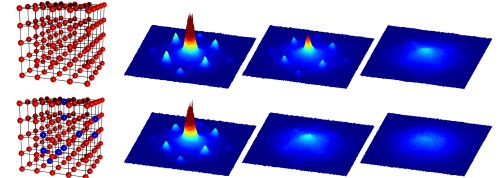
Silke Ospelkaus and colleagues at the Institut für Laserphysik in Hamburg in Germany have done just that, by loading a mixture of ultracold rubidium-87 atoms (fermions) and potassium-40 atoms (bosons) into an optical lattice at a temperature of a few hundred nanokelvin and then abruptly switching off the optical standing wave to see how the gas behaves (figures 1&2). Normally, the bosonic atoms would start to repel each other and form a “Mott-insulator”. But the presence of the fermions, which act as impurities, changes this picture by leading to an attraction between bosons and fermions (Phys. Rev. Lett. 96 180403).

“Such impurity physics is important in many condensed-matter systems but also relevant for other areas, including traffic flow and biological systems,” says team member Christian Ospelkaus. “The new system is also a nice analogy for superconductors,” he adds. “The light field plays the role of the crystal lattice, the fermionic atoms act as the electrons [responsible for the superconducting current] and the attractive interactions between the electrons required for Cooper pairing is provided by the presence of the bosonic atoms – much like phonons in a crystal.”

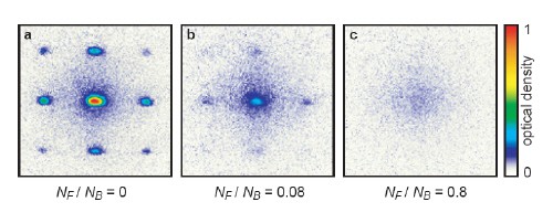
Meanwhile, Tilman Esslinger and co-workers at the ETH Zurich in Switzerland have performed a very similar experiment in which the potassium-40 atoms are “sympathetically cooled” by thermal contact with the bosonic rubidium atoms before being loaded into the optical trap (Phys. Rev. Lett. 96 180402). The Zurich team observed how the presence of fermions in the BEC changed the properties of the initially superfluid bosonic cloud (figure 3). In particular, they noted how the phase coherence – which is the main feature of a BEC – diminished.

“Our work will allow interactions between fermions and bosons in a lattice potential to be studied,” explains Esslinger. “These have strong similarities to electron-phonon interactions in solids and to mixing liquid helium-3 and superfluid helium-4.” Although the Hamburg and Zurich experiments are similar, they differ in the interpretation of the results. Esslinger’s team focus on the coupling between fermions and bosons while Ospelkaus and colleagues look at how bosons behave differently in the presence of fermions.

New look for “Newton’s bucket”

Rotating flows are important in classical fluid dynamics and can produce interesting unstable structures, such as vortices. Since the Earth rotates, such flows are also of interest in geophysics (in the oceans or atmosphere) and in engineering, where they are often found in hydraulic turbo machinery. Moreover, rotating containers can be used to study vortices in experiments and obtain information about natural phenomena such as tornadoes.

The new experiment is an extremely simple example of a “Newton’s bucket” — so-called because Isaac Newton originally used a rotating bucket to discuss the origins of the centrifugal force, which pushes a fluid out against the wall of its container. The present study, performed by Tomas Bohr and colleagues at the Technical University of Denmark in Kongens Lyngby and the Niels Bohr Institute in Copenhagen, is different because the sides of the bucket remain still while only the bottom rotates.

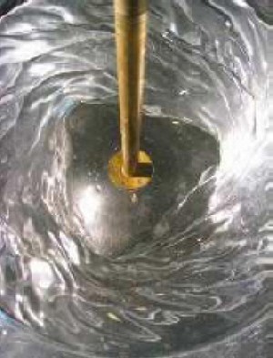
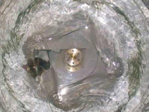
The bucket is made of Plexiglas, is about 20 cm across and contains a rotating plate underneath (figure 1). Bohr and co-workers fill the container with water and set the plate rotating. When the rotation rate becomes sufficiently large, deformations in the form of polygons with up to six corners appear on the surface of the fluid (figure 2).

When the researchers used ethylene glycol, which is about 15 times more viscous than water, they observed three-cornered polygons (figure 3). In some cases, they even saw vortices at the edge of the polygon’s corners (figure 4).

According to the Denmark team, the polygons are new members of a fascinating class of systems where spontaneous breaking of axial symmetry leads to simple stationary or rigidly rotating shapes. Existing members of this family include wavy vortex flows in the “Couette-Taylor” system and classical “Kelvin-Helmhotz-Rayleigh” shears.

The scientists still do not completely understand why the polygons form but now plan to repeat the experiment with buckets of different diameters and fluids that are more viscous. “The variation with these parameters should give us significant information about the origin of the structures,” says Bohr.

Ships shed light on geomagnetic field

Scientists now know that the Earth’s magnetic field is currently decreasing at a rate of about 0.5% a decade. If this trend continues, the magnetic field might reverse so that the North Pole becomes the South Pole and vice versa. Such geomagnetic flips are thought to occur once every 300,000 years or so, with the actual reversal taking thousands of years to complete. However, it is not known whether a decline in the Earth’s magnetic field strength is inevitable.

To help answer this question, David Gubbins and colleagues at Leeds University collected old navigational data from ships’ log books, dating from 1590 to 1840.This data mainly consists of magnetic field directions from the ships’ compasses. The team then used this data to reconstruct the Earth’s magnetic field strength during this time.

The researchers calculated that the “dipole Gauss coefficient”, which is proportional to the Earth’s dipole moment, fell by about 2 nanoTesla per year between 1590 to 1840, which is significantly smaller than the decrease of 15nT per year after 1840. These results show that the magnetic field strength was relatively stable from 1590 to 1840, and has steadily fallen by about 5% each century since then (see figure). Finally, the team also examined the difference in the magnetic field’s structure at the Earth’s core-mantle boundary before and after the mid-1800s from paleomagnetic intensity data. They found that the most recent decline in magnetic field strength most likely comes from an area of reversed flux in the Southern Hemisphere, near Antarctica — a feature that is absent in the 1590-1840 data.

Such changes will present a major challenge to geophysicists, who would like to understand these variations and where they come from in the first place. Scientists believe that our planet’s internal magnetic dynamo is responsible for changes in the magnetic field strength, but the actual mechanisms are not well understood.

How Triton met Neptune

Triton is an unusually big moon and is in fact about 40% bigger than the “planet” Pluto. It is unique among all the large moons in our solar system because it orbits Neptune in the opposite direction to Neptune itself — a so-called “retrograde” orbit. Triton is also an “irregular” satellite that has an inclined, circular orbit around Neptune. It is highly unlikely that the moon formed in such a configuration and was probably captured from elsewhere. But how this happened is a mystery.

Over the years, scientists have proposed several mechanisms to explain how Triton was captured by Neptune. These include the “gas-drag” effect, whereby Neptune’s atmosphere — which was much more extensive than it is today — slowed Triton down enough for it to be captured. Another idea is that Triton may have collided with another satellite near Neptune, causing it to slow down and be captured. However, none of these theories seems to hold up under close scrutiny.

Now, Agnor and Hamilton have proposed a new model that involves a three-body gravitational encounter between a binary and a planet. The physicists say that Triton was originally one of a pair of planet-like bodies, called planetesimals, both orbiting the Sun in the early solar system. Neptune’s gravity then pulled Triton away from its companion when the duo ventured too close to the planet.

The new theory might satisfy two important conditions that should have been present when the capture occurred. The first is that the protoplanetary disk from which Neptune formed must have contained a large number of Pluto-sized objects. The second is that a significant fraction of the large objects in this disk must have been binaries. Indeed, scientists recently discovered that up to 15% of Kuiper-belt objects are binaries.

“We’ve found a likely solution to the long-standing problem of how Triton arrived in its peculiar orbit,” says Agnor. “In addition, this mechanism introduces a new pathway for the capture of satellites by planets that may be relevant to other objects in the solar system.”

Alessandro Morbidelli of the Observatoire de la Côte d’Azur in France agrees and says that the new model could even become a “mainstay for models of the origin of irregular satellites”.

Titan in pictures

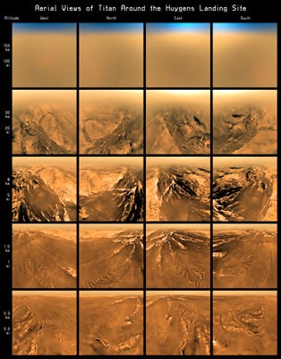
Launched in 1997, NASA’s Cassini spacecraft entered Saturn’s orbit in July 2004. In January 2005, its payload — the ESA’s Huygens probe — successfully landed on Titan after being released from Cassini on Christmas Day 2004. The first movie, which is narrated, runs for about four and a half minutes and shows what the probe saw during the 2.5 hour long descent and touchdown. Another version of this movie is unusually accompanied by a recording of Beethoven’s Piano Concerto no.4 (please see “Related Links”).

“At first, the Huygens camera just saw fog over the distant surface,” explains Erich Karkoschka, who is a team member at the University of Arizona and creator of the movies. “The fog started to clear only at about 60 kilometres altitude, making it possible to resolve surface features as large as 100 metres,” he says. “But only after landing could the probe’s camera resolve little grains of sand millions and millions of times smaller than Titan. A movie is a perfect medium to show such a huge change of scale.”

A second film is more technical and contains detailed text and graphics to explain how Titan looked to the probe during the descent and landing. Different music, modern this time, has also been added to represent the different data sets collected.

“These movies really demonstrate that the Huygens camera was very well designed for the job,” says Jean-Pierre Lebreton, Huygens project scientist and mission manager at the ESA. “They show so many different details of a landscape that covers only a tiny fraction — one-thousandth — of Titan’s surface. This makes me dream of what a possible future mission to Titan may return of this wonderful and fascinating Earth-like world.”

The Cassini spacecraft will continue to orbit Saturn for another two years and its next fly-by to Titan will be on 20 May this year.

Cyclic universe could explain cosmological constant

The cosmological constant, or Λ, was first introduced by Einstein in 1917 to explain why the universe did not appear to be expanding. Edwin Hubble later showed that the universe was expanding, causing Einstein to call the constant his “biggest blunder”. But when scientists first measured a value for Λ in 1998, they found it had a tiny, positive value — indicating that acceleration of the universe is speeding up.

However, it is unclear why this value is an incredible 120 orders of magnitude smaller than would be expected if the universe formed under the “standard” Big Bang theory. Solving this mystery is one of the most important challenges in cosmology today.

Physicists have proposed several theories to explain why Λ is so small. One of the most popular — the “anthropic principle” — states that Λ is randomly set and has very different values in different parts of the universe (figure 1). We happen to live in a rare region, or “bubble”, where Λ has the value we observe. This value has allowed stars, planets and therefore life to develop. However, this theory is also unsatisfactory for many scientists because it would be better to be able to calculate Λ from first principles.

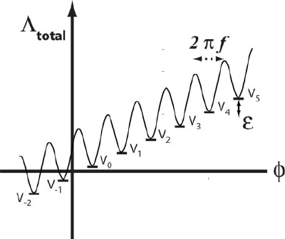
Steinhard and Turok’s new theory assumes we live in a cyclic universe, where each cycle from Big Bang to big crunch takes about a trillion years. It postulates the existence of a long sequence of vacuum states, in which Λ changes in a small series of steps, or cycles, of steadily decreasing cosmological constant. The constant is assumed to start out large and positive and hops down the steps to ever lower values.

Each hop takes longer and longer so that the entire universe spends vastly more time at the lowest positive value of Λ, which we see today, than at any other value (figure 2). The last jump, to a negative value, terminates the cycling behaviour of the universe so that it rapidly ends in a big crunch.

Although a similar model was developed by US physicist Larry Abbot in the 1980s, he showed that the descent to small values of Λ took so long that all the matter in the universe would have completely dissipated during this time, therefore resulting in an empty universe. Steinhardt and Turok have fixed this flaw by combining his model with their cyclic model of the universe. The difference now is that a high density of matter is created at the beginning of each cycle so that the universe is never empty.

“We have proposed a mechanism whereby superstring theory and M theory (our best unified theories of quantum gravity to date) allow the universe to pass through a Big Bang,” Turok told PhysicsWeb. “But more theoretical work is needed to see whether our proposal is fully consistent.”

There will, however, be a way of testing the new theory. According to the standard model of the universe, there was a period of rapid expansion shortly after the Big Bang, known as inflation, that bathed the universe with gravitational waves. A series of experiments are currently underway to detect these waves, which have never been seen before. However, Steinhardt and Turok’s model says the gravitational waves generated if their model is correct would be too small to be detected. So if gravitational waves are found in the next few years, it would rule out their theory.

Hottest topic in physics revealed

The new index is based on the “Hirsch index”, which was devised last year by Jorge Hirsch of the University of California at San Diego as a way of quantifying the performance of individual scientists. Hirsch’s h-index is derived from the number of times that papers by a particular scientist are cited. A scientist with a h-index of 10, say, will have published 10 papers that have received at least 10 citations each. The best researchers should therefore have the highest h-indexes.

Banks has now taken this method a step further by applying the h-index to particular topics or compounds mentioned in the abstract of a paper, rather than to people. A topic or compound with a h-b index of 10 means that there are at least 10 papers on that topic, each of which has been cited at least 10 times. Since some topics and compounds have been around longer than others, Banks divides the h-b by the number of years that papers on that topic or compound have been published. This normalises the result to yield a number, m, which indicates how important a particular topic is today — that is, how many researchers are actively working on it.

Like the original h-index, the h-b index is calculated by searching the ISI Web of Knowledge database, which takes only takes a few seconds. The method involves searching the topic field on the database and then sorting the results in terms of citations. “This is the only method available where you can compare different compounds used in solid state physics or even topics in physics as a whole,” explains Banks.

Banks lists two tables for various compounds and topics according to how big their m and h-b are. Carbon-60 tops the table of chemical compounds, with an m of 5.2, followed by gallium nitride (2.12) in second.

In the list of hot topics, carbon nanotubes are top with an m of 12.85. This is followed by nanowires, quantum dots, fullerenes, giant magnetoresistance, M-theory and quantum computation, which have m numbers of 8.75, 7.84, 7.78, 6.82, 6.58, and 5.21 respectively.

Banks says that an m number greater than three means that a topic is hot. Moreover, a large m number combined with a large h-b (greater than 100) represents a topic that was popular in the past and still is today. Examples of such topics include porous silicon and spin glasses. Finally, a small m but large h-b reflects an older topic that was popular for many years but is now less so, such as perovskites and amorphous silicon.

The new index might help potential PhD students to choose their future area of research, suggests Banks. It could also provide a useful yardstick to compare different fields when awarding funds and grants. However, he warns that his index should not become the only way to assess the importance of a particular subject.

Ice freezes at room temperature

Most surfaces are never smooth and completely flat. If two bodies are brought together, they will not touch over the entire area of apparent contact, but will rather touch over a large ensemble of tiny contacts. Under normal, humid conditions, water vapour can condense out onto these contacts, creating a tiny “capillary bridge”. These bridges tend to make the surfaces stick together and make it harder for them to slide over each other.

However, researchers have not been sure if this is also true when the liquid is confined to small gaps between surfaces. To investigate this problem further, Frenken’s team carried out a series of experiments on an instrument called a “tribolever”, which uses tiny amounts of bending inside a miniature silicon sensor to sense forces as small as 20 picoNewton.

The experiments involved attaching a sharp piece of tungsten wire onto the sensor and carefully scanning it back and forth over the surface of clean, high-quality graphite. The researchers found that icy nanoscale water bridges — lasting for several seconds — formed between the two surfaces at room temperature. In this geometry, the water effectively acted like a glue, and not like a lubricant, joining the two surfaces together.

“Our work provides a new understanding of what happens on the nanometre scale between contacting and sliding bodies,” says Frenken.

The team will now investigate using different materials for the tip and substrate and varying other parameters like temperature and tip speed. They will also study to what extent the ice contributes to friction under practical circumstances.

Plastics go metallic

The new metallic polymer was developed by Kwanghee Lee of the Pusan National University and Suck-Hyan Lee at Ajou University — together with colleagues at the University of California at Santa Barbara. Polyaniline is already widely used as the active component in transistors, light-emitting diodes and photovoltaic diodes because of its good semiconducting properties. It was first found to conduct electricity as long as 1977 and we know that it conducts because electrons move along the backbone of the carbon chain making up the polymer.

However, polyaniline and other conducting polymers do not normally behave as real metals because they are too structurally disordered. Free electrons are therefore “scattered” within the material by the disorder. In metals, in contrast, the electrons are mainly scattered by thermal vibrations of atoms. Since the atoms vibrate less as the metal is cooled, it conducts better at low temperatures

The new polyaniline films show both the optical and electrical properties characteristic of metals. The team made the material by doping it with sulphonic acid and synthesizing it within oily droplets suspended in water. This new technique produced films that are more structurally ordered than polyaniline made using conventional methods.

According to the researchers, the films have a conductivity of about 103 siemens per centimetre at room temperature. Although this is not very high compared to a real metal such as copper, which has a conductivity of 6 x 10⁵ siemens per centimetre under the same conditions, the films are about two and half times more conducting when they are cooled down to 4 Kelvin. Furthermore, the films are shiny and reflect light — albeit in the infrared range of wavelengths. According to the scientists, the optical reflectivity of the plastic in this range fits the model for a simple metal.

But there is a sting in the tail to the new work. Although showing that a polymer can behave like a metal is a real breakthrough, it sets a limit on the conductivity we can expect from such materials in future.

Copyright © 2026 by IOP Publishing Ltd and individual contributors