Page 1729 – Physics World

Home » Page 1729

Shelf life: Simon Singh

What are the three best popular-science books?

Just Six Numbers by Martin Rees. In such a competitive area of science writing as cosmology, the Astronomer Royal found a new angle and his explanations are clear and vivid.

E = mc² by David Bodanis. This is a great book because it makes Einstein accessible to the general public. Some reviewers have criticized it as trivial, but in my opinion it reaches an audience that would not normally even pick up a science book.

Strange Beauty by George Johnson. A far more compelling account of Murray Gell-Mann’s life than his autobiography, this is an important book because Gell-Mann made such huge contributions to physics. As Feynman once said of the man, “The development during the last 20 years of our knowledge of fundamental physics contains not one fruitful idea that does not carry his name.”

What science books are you currently reading?

The Science of Harry Potter by Roger Highfield. This is a book aimed at adults, but the great thing is that it will be picked up by teenagers who will relish the fun ideas contained inside. It has a similar lightness of touch to Highfield’s previous book Can Reindeer Fly? As science editor at the Daily Telegraph, Highfield brings authority and breadth of knowledge to his writing.

What else are you reading?

I have just finished reading Freakonomics, one of the most controversial books of 2005. Economist Steven Levitt and journalist Stephen Dubner analyse various aspects of society with some surprising conclusions. The book’s subtitle says it all: A Rogue Economist Explores the Hidden Side of Everything.

Which popular-science book have you never read, but feel you ought to have tackled, and why?

I do not read enough natural history, although whenever I do delve into this area I am always fascinated. In particular, I should read more of Richard Dawkins’ work. So far I have only read Unweaving the Rainbow and The Selfish Gene, but I look forward to catching up with The Blind Watchmaker and The Ancestor’s Tale.

What advice do you have for physicists who want to write a popular-science book?

Apart from find an interesting story, with some fascinating science viewed from an original angle, my only advice would be to get a good literary agent. If it is the right person, he or she will support you, champion you, enthuse you, act as a sounding board and be a friendly critic.

Cosmology gets precise

Cosmologists face a dilemma. The rise of quantitative cosmology, exemplified by the release of new data in March on the cosmic microwave background from the WMAP satellite (see pp16-19; print version only), threatens to make cosmology a real science at last. But underconstrained speculation is so much fun, as is dodgy philosophy, and both undoubtedly played a major role in attracting today’s practitioners into the art. So what is one to do?

Extending the subject’s bounds well beyond its previous horizons is not a bad start, and there are several serious attempts to keep cosmology speculative. String theory is perhaps not a bad try, wormholes a little more desperate and the overenthusiastic application of the anthropic principle is something of a mini-industry. The rather superficial consideration of infinities and their possible consequences, as well as the introduction of quasi-religious terminology, perhaps go beyond fun into risking intellectual respectability.

Cosmology, the study of the universe writ large, is after all a serious science with a respectable (recent) history of major discovery and some limited explanation. Just a century ago there was no appreciation of the vast size of the universe – though it was well understood to be very old. Its expansion was unknown, the concept of a single origin in the Big Bang was rash pseudo-creationism, and the idea that one could directly observe photons generated when the universe was less than 1% of its present age was absurd. In those days, terms such as dark matter and dark energy would have conjured up images of coalminers rather than philosophers. Developing our current model of cosmology was one of the greatest intellectual achievements of the 20th century – a period in which rather a lot of stunning advances vie for that honour.

The story is well known, though it bears retelling for each new generation. Indeed, the first part of this fascinating and frustrating new book by the distinguished cosmologist Joseph Silk is a rather standard run through the history of modern cosmology. Some parts are superb, in particular the explanation of the meaning of the cosmic microwave background – not surprising, given the major contributions to the subject made by the author. Other parts, especially the description of the consequences of the microwave-background polarization results from WMAP, have already been overtaken by new data, reminding us that precision cosmology is a work in progress – still under development and only part robust science.

Even if the content is familiar, Silk does have an excellent style: he cleverly mixes the basic science with anecdotes about the personalities involved, and is not afraid to make his opinions and criticisms clear. Readers will enjoy a superb description of the abuse of science by the PR departments of major labs; an abuse being re-enacted today as credit for the “discovery” of dark energy, in fact a culmination of half a century of work started by Edwin Hubble and carried forward by Allan Sandage, is claimed by a few latecomers.

Some readers may wish to rush through the introductory overview and get on to the main course. Here Silk adequately introduces some of the more unusual concepts used in modern physics and cosmology, and makes a quick dash through the role of the observer in quantum mechanics. The brief tour of the multiverse is acceptable too, but the really creative and challenging part of the book comes in the now-obligatory philosophical section. Here Silk does substantially better than most of the nonsense served up in recent cosmology books: indeed exposing it as nonsense is something Silk does eloquently and well.

In some of these other recent discussions of the far future and multiverses, one can find statements such as “other intellectual life is inevitable in an infinite universe” and “in an infinite universe eventually everything will happen”. This, without qualification, is nonsense: I can readily imagine an infinite static universe that is infinitely empty, in which infinitely nothing will eventually happen. It is simple to imagine what the authors of such statements intend, but the point of philosophy is intellectual and literary exactness – otherwise such ideas are speculative rubbish.

As another example, it is now a mere truism that scientists abuse the name of God in populist books. In addition to betraying a depressing lack of literary inventiveness, such use of emotionally charged and complex-valued terminology confuses and abuses the trust of the non-expert public. Here Silk rises above such limits, providing a clear and interesting commentary, pulling no punches, and naming names of some of the most egregious offenders. Scientists have no right to smug contentedness when exposing sham, such as through the Sokal “hoax”, if our own community exploits the same mix of gullibility and obscurity. The author’s comments on this issue are trenchant and thoughtful.

Silk raises many interesting ideas in the book, albeit almost all only in passing in a style and at a depth that is more along the lines of a dinner-table conversation between academics than a deep analysis. There is enough here, however, to introduce the reader to the subject of modern cosmology and to the more interesting philosophical ideas that arise in that study. The style and level are appropriate to allow interested readers to start to think more deeply for themselves about these complex and fascinating concepts.

WMAP data put cosmic inflation to the test

While gazing upwards at the night sky you could be forgiven for thinking that the universe is a rather complex place. From elaborate constellations of nearby stars to the faint glow of light from the spiral arms of our galaxy, structure is visible in every direction you look. And were you to peer through the world’s largest telescopes you would find a hierarchy of galaxies grouped into clusters, superclusters and super-superclusters hundreds of millions of light-years across. But to cosmologists, this clumpy nature of matter is a mere distraction.

On the largest cosmic scales, the universe is astonishingly dull. We know this courtesy of the cold sea of radiation that permeates the most distant reaches of the universe: the cosmic microwave background. Discovered serendipitously in 1965, this radiation contains unique clues about the nature and content of the cosmos because it came from an epoch when our universe was just a few hundred thousand years old.

A matter of scale

Its most remarkable feature, however, is its near lack of any features at all! For almost 30 years following its discovery, the only thing we knew about the cosmic microwave background was its temperature – a chilly 2.725 K. And this temperature is the same to better than a part in 10,000 no matter which direction in the sky we measure. So where did the structure in the universe – from which the Sun, the Earth and we ourselves ultimately descended – come from?

Cosmic explorer

Cosmologists are now able to address fundamental questions such as this from precision measurements of the cosmic microwave background. The first such data came courtesy of the COBE satellite in 1992, revealing miniscule fluctuations in the temperature of the microwave background as a function of position in the sky. And in 2003 the Wilkinson Microwave Anisotropy Probe (WMAP) gave cosmologists a crisp new view of this temperature anisotropy. Three years on, after a painstaking analysis that allowed the WMAP team to map the polarization of the cosmic background radiation across the sky, we are now in a position to put the standard model of cosmology through its toughest test to date.

A bold idea

The cosmic microwave background (CMB) was born when the universe was about 380,000 years old. Before this time, space was filled with a hot plasma of electrons and light nuclei, which meant that light could not travel very far without being scattered. But as the universe expanded, the plasma cooled enough to allow neutral atoms to form. This “decoupling” of matter and radiation suddenly enabled photons to travel across space largely unimpeded, their wavelengths being stretched over time to produce a faint glow of radiation in the microwave region that we can detect today.

In the early 1980s, in an attempt to explain the mind-boggling uniformity of the CMB, theorists came up with a bold concept called inflation. The idea was that the universe underwent a period of enormous growth when it was just 10^-35 s old, during which it expanded by a factor of at least 10²⁶ in a fraction of a second. Inflation could therefore account for the uniformity of the CMB because it proposes that the portion of the universe we observe today inflated from a tiny region that was presumably in thermal equilibrium. Without inflation, regions in opposite directions of the sky could never have been in contact – let alone thermal equilibrium.

Another consequence of inflation is that any previously existing curvature in space-time would have become immeasurably small after the exponential expansion, thereby accounting for the flat, Euclidean geometry of the present-day universe. Perhaps most remarkably, however, inflation offers an explanation for the clumpiness of matter in the universe: quantum fluctuations in the mysterious substance that powered the expansion would have been inflated to astrophysical scales and therefore served as the seeds of stars and galaxies.

Inflation is a key component of what is known as the standard cosmological model, but so far it has been very difficult to put the idea to the test directly. The tiny temperature anisotropy in the CMB provides a way to do this, since it is linked to the initial quantum fluctuations in the “stuff” that powered inflation. However, before we can extract useful information about these fluctuations, we need to understand other effects that contribute to the observed temperature anisotropy.

The most prominent effect is that of weak, low-frequency sound waves in the primordial plasma. A direct product of the initial quantum fluctuations, these waves “froze out” when matter and radiation decoupled 380,000 years after inflation to leave a distinctive oscillatory signature in the CMB anisotropy. Another important effect is that of secondary scattering, whereby on their journey across the universe some of the CMB photons scattered off free electrons in gases that were heated by the first stars. In addition to reducing the amplitude of the anisotropy signal, these interactions would have polarized the photons. Physicists have therefore been eager to measure the polarization of the CMB across the whole sky, which would give us both a better idea of how much attenuation took place and when the first stars formed.

Fortunately, the physics of these separate contributions to the CMB anisotropy is quite well understood, so it is straightforward to disentangle them from the initial quantum fluctuations. In order to do so, however, we need high-resolution measurements of the temperature and polarization of the CMB over the full sky – something that is now coming to fruition.

Anisotropy observations

In April 1992 a team led by George Smoot at the University of California at Berkeley and Chuck Bennett at NASA’s Goddard Space Flight Center announced the first detection of anisotropy in the CMB temperature. Using the COBE satellite, they found variations in the temperature of roughly one part in 100,000 (which equates to about 30 μK) from point to point across the sky. The wonderful map of the fluctuating microwave background – which Smoot famously likened to “seeing the face of God” – had three major implications for cosmology.

First, it showed that nature has been kind to us, since the amplitude of the anisotropy is large enough to stand out above the microwave emission from our own galaxy (provided we look in the direction away from the galactic plane). Second, the measurement fixed the amplitude of the initial quantum fluctuations for the first time. But since inflationary models do not specifically predict the amplitude of the initial fluctuations, this measurement did not directly test inflation as the source of the fluctuations. The third important implication of the COBE data, however, was that they provided a rough test of inflation by constraining a parameter called the scalar spectral index.

The scalar spectral index, n_s, measures the relative strength of the temperature anisotropy on small and large angular scales. As such, it corresponds to the slope of the angular power spectrum – which plots the temperature anisotropy as a function of angular scale – once its oscillatory features have been removed (see figure). Before inflation was introduced, theorists argued that the spectral index needed to have a value of unity to produce the correct relative abundance of stars, galaxies and clusters of galaxies. This corresponds to a flat line in the angular power spectrum. Although today’s inflationary models predict a range of values for n_s, all of which are close to unity, the simplest models predict a value slightly but measurably less than one.

Due to its limited angular resolution, COBE was only able to measure the anisotropy at large angular scales, which made it difficult to measure n_s precisely. Throughout the 1990s, however, several sophisticated ground- and balloon-based experiments were carried out to measure the CMB temperature anisotropy with finer angular resolution. While these experiments could only observe relatively small patches of the sky, their results began to refine the measurement of n_s, and to test the other major prediction of inflation: the flatness of the universe, which is determined by the position of the first acoustic peak in the angular power spectrum.

Then, in June 2001, NASA launched the WMAP satellite, which was designed to produce full-sky maps of the CMB anisotropy with higher sensitivity and resolution than ever before. Results from the first year of WMAP observations were released in February 2003. Among other things, these allowed researchers to conclude that the universe is 13.7 ± 0.2 billion years old and that its geometry is Euclidean to within 2% (see “The cosmic microwave background” Physics World April 2003 pp27-32). The first-year data also corroborated the standard “cold dark matter” model of the universe, suggesting that the relative abundances of ordinary matter, dark matter and dark energy in the universe are 4.4%, 24% and 72%, respectively.

Three-year WMAP results

In March the WMAP team announced results based on three years’ worth of WMAP observations, which includes the most precise measurements of n_s to date. One of the key features of the new data is that they have enabled us to measure the polarization of the cosmic microwave background. For an electromagnetic wave propagating along the z-axis, its polarization state is described by the relative amplitude and phase of the x and y components of the oscillating electric field. Specifically, if the line of sight from the observer to a free electron is the z-axis and the CMB photon has an intensity asymmetry in the x-y plane, then the radiation scattered in the z-direction will be polarized – much as sunlight is polarized when viewing the sky at right angles to the Sun.

There are two periods in the history of the universe during which free electrons were available to polarize CMB photons: first at the epoch of decoupling, and then again at the epoch of “reionization” – a few hundred millions years after decoupling – when the first stars ionized the surrounding gas. The polarization signal produced at decoupling only appears at small angular scales less than about 1°, while that produced by the reionized electrons occurs on angular scales of tens of degrees because these electrons are much closer to us.

Thus, by measuring the large-scale polarization of the CMB we can measure the “optical depth”, τ, of the reionized gas – which gives the probability that a CMB photon was scattered by a reionized electron on its trip across the universe. A by-product of this scattering is that it suppresses the amplitude of the small-scale temperature anisotropy by a factor of e^-2τ, which is important because it gives cosmologists a new handle on disentangling the effects of acoustic oscillations and secondary scattering from the primordial fluctuation signal produced by inflation.

One of the most daunting challenges for the WMAP team has been to measure the temperature anisotropy of the polarized photons, which, at about 0.1 μK, is over 100 times weaker than the unpolarized signal. To reach such exquisite precision, which is 50 times better than the original requirement for the WMAP mission, we had to rewrite the data-processing algorithms twice and construct an elaborate “covariance matrix” in order to measure how the noise in a single sky-map pixel correlates with the noise in every other pixel. The full-resolution sky map contains over three million pixels, but we had to use a lower resolution of 3072 pixels to make the matrix tractable. It was also crucial to have several independent years of data (WMAP repeats a full-sky survey every year) in order to perform vital cross-checks of the results.

The final analysis of the full-sky polarization maps suggests that the optical depth produced by reionized electrons is 9 ± 3%, which implies that the first stars formed roughly 400 million years after decoupling. In contrast, the first-year WMAP data put this event at about 200 million years. The new determination of the optical depth has also allowed us to refine our measurement of the scalar spectral index to be n_s = 0.951 ± 0.016, compared with the first-year estimate of 0.99 ± 0.04.

Thus, for the first time we have evidence based solely on CMB data that the spectral index prior to inflation is significantly different from the scale-invariant value of unity, which had been long advocated on the basis of somewhat ad hoc arguments. In contrast, simple models of inflation in which the cosmic expansion is driven by a single “scalar field” predict that the spectral index should be measurably less than one and in the range observed by WMAP.

Grand unification

The era of precision cosmology is well under way, and is now reaching the realm of precision tests of inflation. But there is one more prediction of inflation that remains to be verified. According to Einstein’s general theory of relativity, the fluctuations produced by inflation are accompanied by variations in the curvature of space-time, which include gravitational waves. Since CMB photons gain or lose energy as they traverse the associated gravitational potential wells, gravitational waves would also contribute to the temperature anisotropy.

The most compelling test of inflation would therefore be to unambiguously detect these relic ripples in space-time. Crucially, the amplitude of the gravitational-wave signal depends on the energy scale of inflation, so detecting it would significantly constrain models of what actually powered inflation. Since the unpolarized CMB signal arises from both the density- and gravitational-fluctuation sources, we need to somehow determine the ratio of the two contributions.

At present our only handle on this comes from the shape of the unpolarized anisotropy spectrum, but that information does not unambiguously determine the ratio. However, if inflation occurred at the “grand unification” scale (about 10¹⁵-10¹⁶ GeV), then the gravitational-wave signal could be inferred indirectly from observations of the CMB polarization. Specifically, gravitational waves would instil a unique vortex-like pattern in the polarization that might be detectable with a well-designed polarization experiment. We therefore have the tantalizing possibility of probing physics at energy scales several orders of magnitude higher than are possible with any terrestrial particle accelerator!

A recent study of inflation by Latham Boyle of Princeton University and co-workers shows that if the scalar spectral index n_s is indeed greater than 0.95 – i.e. in accord with current measurements – then the ratio of the gravitational-wave and density contributions to the CMB anisotropy is greater than 0.01, otherwise the inflationary model is “unnaturally fine tuned” (www.arXiv.org/abs/astro-ph/0507455). Although very small, Boyle and colleagues say that such a signal should be detectable in proposed CMB polarization experiments and direct gravitational-wave searches. So, there is reason to be optimistic about the prospects for detecting such a signal. To date, inflation has passed a number of very significant tests, and the detection of a gravitational wave background would be another notch in its belt.

• map.gsfc.nasa.gov

Antarctica unravelled

Antarctica is the world’s last great wilderness. Desolate, cold and largely unspoilt by humans, the continent provides a natural habitat for penguins, seals, whales and other wildlife. It is also home to the largest reservoir of fresh water anywhere on Earth, in the form of a vast sheet of ice that covers almost all of its land. Bounded by icy peaks, dry valleys and the southern oceans, this sheet plays a key role in the Earth’s hydrological cycle.

Every year a volume of water equivalent to the upper 7 mm of all of our planet’s oceans falls as snow on the Antarctic ice sheet, while a roughly equivalent amount of ice slips into the sea via glaciers. But the ice sheet is seldom in a state of balance. From one ice age to the next, and from one season to the next, the amount of snow arriving differs from the amount of ice leaving, causing parts of Antarctica’s frozen reservoir to be alternately drained and replenished. When the ice sheet grows, global sea levels fall; when it shrinks, sea levels rise.

Given that Antarctica is exposed to the atmosphere and oceans, sudden changes in the Earth’s climate can also alter this balance. But because Antarctica is a largely frozen environment, its ice was expected to respond only slowly to the recent increase in global temperatures – which have climbed 10 times faster in the 20th century than at any other time in the last 1000 years. Now, however, satellite observations tell a different story. Coastal glaciers are accelerating and thinning at various places around the entire continent, and it seems that the vast quantity of heat delivered by the Earth’s gradually warming oceans may be to blame.

Collapsing continent

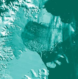
The first cracks in Antarctica’s icy armour appeared in the mid-1990s. Massive ice shelves floating in bays around the Antarctic Peninsula – a narrow mountain chain that extends northwards towards South America – began to disintegrate. Geological records suggest that the largest of these shelves, the Larsen ice shelf, had occupied a bay about the size of Scotland for over 5000 years. But in 1995, and again in 1999, vast sections as large as London detached and floated away in a matter of days.

This contemporary example of abrupt climate change even played a cameo role in the blockbuster movie The Day After Tomorrow. But, on that occasion, Hollywood was not guilty of melodrama. While the film’s computer-generated imagery showed a single crack splitting the shelf in two, the reality was far more dramatic: each section shattered into millions of icebergs. Should the current warming trend continue, the rest of the Larsen ice shelf could well fragment too.

1 Crunch time

Although the collapse of the Larsen ice shelf was initially studied using simple satellite photographs (figure 1), its consequences have only recently been revealed with the aid of more sophisticated techniques. In particular, radar measurements from space have allowed physicists to monitor changes in the thickness and flow of the ice. Thanks to these techniques, we now know that the tributary glaciers that fed the Larsen ice shelf while it was intact have thinned and started to move faster since the collapse, dumping more ice into the oceans and raising the world’s sea levels.

It is a worrying finding. If the same course of events were to take place in other parts of Antarctica, the changes in global climate expected over the coming century would trigger an unprecedented rise in sea levels. In the most extreme scenario, this could flood cities like London, and threaten the warm climates of northern Europe (see “Antarctica explored”). We therefore urgently need to understand in more detail how Antarctica will respond to global warming.

Journey south

Antarctica is a vast continent covering an area of over 12 million square kilometres – about 50 times the size of the UK – and a permanent ice sheet covers 98% of its land. This ice sheet, which is up to 4 km thick in places, is bisected by a chain of mountains. On the eastern side, the ice sheet rests on bedrock that lies above sea level; if the ice sheet were removed, the rock would form an island. On the much smaller, western side of the mountain range, the ice sheet lies on the sea floor – an unstable configuration. The entire sheet is drained through giant glaciers up to hundreds of kilometres long that channel ice from the cold interior of the continent towards the southern oceans.

2 Antarctica explored

The chief goal of Antarctic experiments in recent years has been to establish whether the ice sheet is growing or shrinking, since even tiny differences between the amounts of snowfall and glacier discharge would lead to large changes in global sea levels. Although we now have accurate charts of Antarctica, the first of which were drawn by the 19th-century mariners who first sighted the continent, we can only determine the total volume of the ice sheet by knowing how thick it is. The overland expeditions of Amundsen and Scott to the South Pole were of little help in this context, and it was not until the late 1950s that the first reliable thickness estimates were made (figure 2). Based on data collected during the Commonwealth Transantarctic Expedition of 1958, Ed Thiel of the University of Minnesota calculated that the Antarctic ice sheet had a volume of 24 million cubic kilometres, about 20% short of today’s best estimate.

At the time of the last ice age, about 20,000 years ago, Antarctica was much bigger than it is today, and in places its coastline was 500 km farther north. However, it has proved extremely difficult to determine whether the ice has stopped retreating or begun to expand once again. The first attempts to answer this question were made in the 1960s, when scientists carried out field surveys to measure the rate at which the mass of the Antarctic ice sheet was changing. But these early results have proved unreliable. The sheer size of Antarctica – over 5000 km wide in places – bars any realistic sampling at ground level, so satellite measurements are the only way forward.

Balancing the books

There are just three practical ways to measure changes in the mass of an ice sheet. The first approach, known as “balancing the mass budget”, involves estimating how much snow falls on the continent and then subtracting the mass of all the ice leaving via glaciers plus all the water leaving via run-off (negligible in Antarctica). The second technique involves estimating the volume of the ice sheet, while the third involves measuring its gravitational attraction.

Down under

Glaciologists have traditionally favoured the mass-budget method, which is most easily determined for individual glaciers because ice is channelled across well-defined drainage catchments, rather like water in a river network. Measurements of net accumulation (snowfall minus any run-off) are usually integrated across the entire glacier, while ice discharge is computed across a line at the base of the glacier near to its terminus.

In recent years, the mass-budget method has improved through the growing use of interferometric synthetic aperture radar (InSAR). This satellite-based technique has allowed researchers to make precise measurements of glacier speed, thereby reducing the uncertainty in mass loss. The main problem with the mass-budget method is that it relies heavily on sparse historical records for snowfall, and the technique is still hampered by a lack of accurate snowfall and ice-thickness data.

The second way to measure variations in the mass of an ice sheet – the volume-change method – involves recording small fluctuations in ice elevation over time and attributing any differences to either a change in snowfall or ice mass. In practice, however, this technique only works well if data are obtained over large areas and sampled at frequent time intervals. The method was not therefore particularly successful until data from radar altimeters aboard the European Remote Sensing (ERS) satellites were obtained in 1991.

These instruments transmit pulses of microwaves towards Earth and record the time taken for the scattered radiation to return to the satellite. Knowing the speed at which the microwaves travel through the Earth’s atmosphere, the travel time allows the height of different parts of the Antarctic ice sheet to be determined (see “Physics on ice”). The advantage of satellite altimeters over those on, say, planes is that they pass repeatedly over the same region of Earth, which allows researchers to determine how the volume changes over a particular region. The major uncertainty comes when converting this volume change to a mass change, which requires an accurate estimate of the relative densities and quantities of ice and snow. Volume-change calculations are therefore usually performed at the scale of individual drainage basins, where some advance knowledge of meteorological (snow) or dynamical (ice) fluctuations is available.

The final method for measuring the change in mass of the Antarctic ice sheet relies on precise measurements of the Earth’s gravitational field obtained by, for example, the Gravity Recovery and Climate Experiment (GRACE). Launched in 2002, the GRACE mission involves monitoring small fluctuations in the orbits of a pair of satellites flying in tandem. These tiny movements, which are caused by changes in the Earth’s gravitational field across different parts of the planet, can be used to estimate changes in the total mass of the planet’s water.

Isolating changes in the mass of the Antarctic ice sheet is not easy using this technique, particularly because the mass of rock beneath Antarctica has been changing since the last ice age as the Earth’s outer shell adjusts slowly to a reduction in ice loading. However, Isabella Velicogna from the University of Colorado in the US has recently produced the first comprehensive survey of the entire Antarctic ice sheet using data from GRACE. Reported in Science in March, she concluded that the ice sheet had lost mass at a far greater rate over the past three years than during the preceding decade, mostly from West Antarctica. Her finding – an annual mass loss of 139 gigatonnes (139 × 10¹² kg) – was surprising given that the last report of the United Nations’ Intergovernmental Panel on Climate Change (IPCC) had predicted that Antarctica would probably gain mass during the 21st century due to increased precipitation in a warming global climate.

It is not easy to say which of the three techniques has provided the best measure of Antarctic mass balance because they each measure the continent over different scales of distance and time. The volume-change method suggests that the ice sheet is increasing by 27 ± 29 gigatonnes per year; the mass-budget method says it is falling by 26 ± 37 gigatonnes per year; while the gravity method indicates it is falling by 139 ± 73 gigatonnes per year, although much of this difference can be accounted for by the fact that each technique surveys different areas of the continent.

Taken together, however, the results suggest that Antarctica could be making global sea levels rise by as much as 0.1 mm a year or fall by as much as 0.4 mm a year. Although these figures may sound vague, the uncertainty is far less than for results from past glaciological surveys. The results have also helped the IPCC to understand the recent increases in global sea levels, which rose by a staggering 18 cm during the 20th century.

A cautionary finding was announced by Matthew Lythe of the British Antarctic Survey in 2001. He re-examined information about the continent’s bedrock that had been obtained through extensive geophysical surveys of the previous 30 years by researchers from the Scott Polar Research Institute, the Technical University of Denmark and the National Science Foundation in the US. Between them, these institutes had surveyed almost a third of the continent via aircraft sorties, and had measured properties such as the thickness and elevation of the ice. By simply constructing a map of ice thickness, Lythe calculated that the ice sheet has a volume of 30 million cubic kilometres. Given that four-fifths of this rests above sea level, he concluded that global oceans would rise by a staggering 57 m if the ice were to rapidly melt.

Runaway train

Measurements of glacier speed, which are essential for mass-budget surveys, began centuries ago when early geographers charted the motion of Alpine glaciers on foot. However, large-scale changes could only be monitored with ease following the development of remote-sensing techniques in the 1950s. In Antarctica the first such attempts involved taking photographs of the continent and then noting from them the rate at which crevasses and other features on the glacier surfaces were shifting – a method that is still employed today with data from satellite cameras. In 2004, for example, Ted Scambos of the National Snow and Ice Data Center in Colorado, using images from NASA’s Landsat satellites, found a sixfold increase in the speed of glaciers moving into a bay that appeared after the Larsen ice shelf had collapsed. Presumably the ice shelf was exerting pressure on the glaciers above it, so that when it collapsed the resistance to flow was removed and the glaciers started moving faster.

These and other events were also recorded by Eric Rignot of NASA’s Jet Propulsion Laboratory (JPL) in 2002 using InSAR (see “Physics on ice”). By charting the position of its grounding line over a four-year period between 1992 and 1996, he also revealed that the Pine Island glacier in western Antarctica was retreating at a rate of 1.2 km per year. Since then, Rignot and Ian Joughin (then also at JPL) have surveyed a further 33 Antarctic glaciers – which drain about 60% of the ice-sheet area. By comparing the discharge from the glaciers with estimates of their inland snow accumulation, Rignot concluded that western Antarctica was losing 48 km³ of ice each year, enough to raise global sea levels by about 0.12 mm. But the errors for East Antarctica were too large to give a reliable sign for the trend, while the scarcity of snowfall and glacier-thickness measurements still limit the accuracy of InSAR mass-balance estimates today.

Inflation and deflation

When the European Space Agency launched its satellite ERS-1 in 1991, a race began to determine volume changes of the Antarctic ice sheet using data from its radar altimeter – the first such device to survey polar regions. Since the satellite repeated its orbit around the poles every 35 days, researchers were able to distinguish changes in the height of various points on the Antarctic ice sheet over time from changes in the slope of those locations.

Using this technique, Duncan Wingham of University College London concluded in 1998 that in the four years to 1996 some three-quarters of the Antarctic ice sheet had shrunk by, on average, 68 km³ a year. Once this much ice ends up in the sea, it causes global sea levels rise by about 0.16 mm. These estimates have since been backed up by measurements from Jay Zwally of the Goddard Space Flight Center and Curt Davis of the University of Missouri, who have performed similar surveys over longer time periods.

But why had the sheet shrunk? There are two possible answers – either less snow fell in Antarctica when the measurements were made or there was a surplus outflow of ice into the sea via glaciers. The problem is that the two processes fluctuate on markedly different timescales: snowfall in Antarctica commonly varies on roughly decadal timescales, whereas glacier flow imbalances often persist for centuries or more. So if the thinning were due entirely to reductions in snowfall, the data are unlikely to have given a useful indication of the trend of the ice-sheet mass. On the other hand, if the changes were due to a glacier-flow imbalance, the measurements probably do reflect a long-term effect.

The other difficulty with interpreting altimetry results is that volume changes can only be converted into mass changes by ascribing a density, and the density of snow is one-third that of ice. So if the density prescription is wrong, the mass change will be in error. In 2001 I managed to assign a density of ice to the volume losses in western Antarctica by studying satellite radar records of the Pine Island glacier, which revealed that the ice was thinning only where it was flowing most rapidly. In all, the glacier was losing about 8 gigatonnes of ice each year, and the study provided the first evidence that a long-term disturbance to glacier dynamics was widespread in this sector of Antarctica.

Since then Tony Payne from Bristol University in the UK has taken a closer look at the glacier to investigate the origins of today’s disturbance. Using a computer model of the glacier flow, he showed in 2004 that the thinning can be explained if the ocean at the terminus of the glacier is about 0.5° above freezing, which would trigger a “wave” of thinning travelling upstream. Indeed, there is evidence for such a change, with temperature profiles recorded by Stan Jacobs of the Lamont Doherty Earth Observatory in 1996 showing that a warm current of water circulates in front of the glacier.

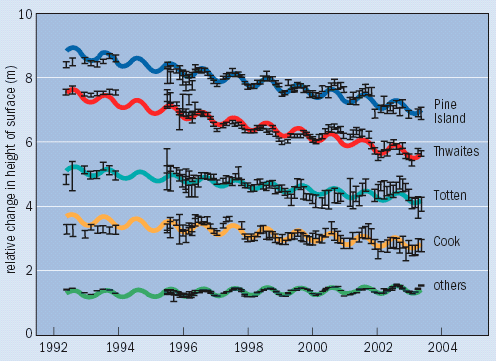
The most recent satellite observations show that three other glaciers in Antarctica – in addition to the Pine Island glacier – are retreating in the same way, even though the Antarctic ice sheet is growing overall at a modest rate (figure 3). The growth in the size of the main ice sheet is due to a short-term increase in snowfall, whereas the thinning is due to a longer-term acceleration of glacier flow, possibly triggered by warming oceans. If ocean temperatures continue to warm, as the last report of the IPCC projects, these glaciers could begin to shed mass at an even faster rate.

Challenges for the future

3 On thin ice?

The past few years have witnessed a colossal increase in our understanding of Antarctica, thanks to the constellation of microwave sensors that now orbit Earth. But there is still much that remains uncertain. Although estimates of the ice-sheet mass balance determined from all three different measurement approaches concur that western Antarctica is losing mass and that eastern Antarctica is close to being in balance, individual results for many glaciers show poor agreement. This stems largely from the accuracy of ancillary datasets, and without better constraints on such things as ice-thickness and snowfall records we cannot hope to get a final answer.

Today, we rely on terrestrial measurements for each of these parameters, and there is no realistic prospect that our capacity to survey these manually will substantially increase. But it is possible to sample each remotely, and radar engineers are making every effort to develop remote systems that are up to the task. Today’s airborne microwave radars can resolve annual ice layers to depths of up to 50 m – often representing over a century of snowfall – and recent work by Robert Hawley of the Scott Polar Research Institute shows similar results may be obtainable from space.

Unfortunately, the outlook for space-borne ice-thickness measurements seems less certain; although a satellite-mounted ice-penetrating radar is technically feasible, the required bandwidth is already employed for telecommunications, and it is difficult to envisage science outflanking commerce in that conflict. A team lead by Prasad Gogineni of the University of Kansas is, however, aiming to avoid such a confrontation by developing autonomous aircraft on which scientific payloads can be flown, with the long-term goal of mapping the geometry of bedrock beneath all of Antarctica.

Our ability to predict future changes in sea level remains compromised by a lack of satellite data from the coastal sectors of Antarctica, where much of today’s changes have taken place. Current satellite altimeters have coarse Earth footprints – about 10 km across – and when terrain becomes rugged they fail to record echoes. The current generation of satellite synthetic-aperture radars struggle to record the fast ice motion in these sectors, and so direct measurements of flow imbalance can no longer be made. Although there is no future InSAR mission on the horizon, there is the prospect of a fine-resolution satellite altimeter within the coming years.

The scientific case for the European Space Agency’s CryoSat mission, which was lost due to a rocket failure shortly after it took off last October, remains, if anything, more compelling today than in 1998 when the mission was first conceived. CryoSat offered the prospect of measuring changes in elevation with a spatial resolution an order of magnitude better than today’s instrumentation – just what is required to survey coastal Antarctica. Fortunately, ESA has recently approved a follow-on mission, Cryosat 2. One thing is certain: without new space instrumentation, the mysteries of glacier drawdown at the coast of Antarctica will remain unsolved.

At a Glance: Antarctica

Antarctica is about 50 times the size of the UK, and 98% of its land is covered by a permanent ice sheet that is up to 4 km thick
The continent contains 90% of the Earth’s fresh water, which falls as snow, leaves via glaciers and causes major changes in global sea levels
Large chunks of the Antarctic ice sheet have disintegrated in recent years and the coastal ice is retreating in places, quite possibly due to global temperature rises
Knowing the electromagnetic response of snow and ice, physicists can measure the thickness and therefore volume of the ice sheet using microwaves
The most promising way to monitor the profound changes in Antarctica is to perform such radar surveys by satellite, which can also tell us about the ice sheet’s speed and thickness change

Antarctica and climate change

What would happen if the Antarctic ice sheet were to collapse entirely? First, all the world’s oceans would rise by a staggering 57 m – enough to inundate 18 of the 20 most-populated cities on Earth, including New York and London. Moreover, the sudden input of icy cold waters could disturb patterns of global ocean circulation and threaten the uncommonly warm climates that northern Europe experiences today.

Although we are not sure what will happen in the future, we do know that the Earth’s sea levels rose by some 18 cm during the 20th century, most of which was due to thermal expansion rather than to any change in mass. In fact, as temperatures rose, more snow fell on Antarctica. The continent therefore acted as a counterbalance to any increase in mass, soaking up the equivalent of about 1 cm of water over the entire century. This is such a small fraction (about 5%) of the water that passes through Antarctica each year that climatologists assumed that the ice sheet is relatively stable to climate change.

But if – as is widely expected – our planet’s climate warms faster during this century than the last, then the continent may contribute much more in the future to rising sea levels. Indeed, a handful of large Antarctic glaciers are already rapidly retreating, which could draw down inland ice into the sea even faster, particularly if the world’s oceans warm up as expected. In little more than a few decades the ice sheet could then switch from growth to overall decay and, in turn, cause sea levels to rise.

Physics on ice

One of the most useful ways to study Antarctica is to examine the electromagnetic properties of snow and ice using microwaves and radio waves. The ice is formed from snow that falls on the surface of a glacier and presses down on itself. Seasonal fluctuations in temperature and precipitation create annual layers of ice called “isochrones”, each of which submerges over time. The way in which electromagnetic radiation interacts with these layers depends on their precise geometry and structure. By studying that interaction, we can gain valuable insights into the structure of the ice. Microwaves and radio waves are of particular interest because their wavelengths (0.1 mm-1000 m) are similar to those of natural snow structures.

Provided they are of high enough energy and frequency, radio waves can penetrate even the thickest Antarctic ice – up to 4 km in places. Most measurements are carried out by sending a radio signal from a plane. Typically, the strongest echo comes from the interface between the ice and bedrock, but intermediate reflections from internal layers in the ice are commonly seen too. The layers, which were first observed by Gordon Robin of the Scott Polar Research Institute in Cambridge in 1964, indicate changes in the density, conductivity and flow properties of the ice. They therefore provide valuable information about how ice builds up and deforms over time.

But the true importance of radar techniques for glaciology became clear when the first low-frequency microwaves were directed towards ice from space in the late 1970s through the technique of radar altimetry. Having shorter wavelengths than radio signals, microwaves penetrate only tens of metres within a typical snow-pack. Although the echoes from a glacier’s surface are distorted by scattering from layers buried at depth, these effects can be accurately unscrambled using a theoretical model that was originally developed in 1977 by Gary Brown of Virginia Polytechnic Institute and is still in use today. The net result is that satellite radars can repeatedly record the height of ice-sheet surfaces with incredible precision – to within a few centimetres in the most-favourable areas.

Another vital tool in glaciology is interferometric synthetic aperture radar (InSAR), which was pioneered in the early 1990s by Richard Goldstein and colleagues at NASA’s Jet Propulsion Laboratory in California. This technique involves recording the phase change of the microwaves as they bounce off objects on the ground. Although the electromagnetic phase of an individual SAR image is incoherent, the phase difference between two SAR observations of the same scene recorded from satellite locations close together in space can be strongly coherent, provided the target characteristics do not change much between the two observations. This interference signal, or interferogram, is a measure of the component of ground displacement in the line of sight of the radar beam relative to the spacecraft. By taking measurements repeatedly over the same spot, it is a relatively straightforward procedure to work out how fast the ice is moving.

InSAR has been widely employed in glaciology to chart both ice motion and the location of glacier grounding lines (the junction between ice, bedrock and the ocean, where ice begins to float). While a single interferogram is sensitive to both the geometry and deformation rate of the target surface, several images can be combined to isolate either signal. As Goldstein predicted, the technique has since been used to map the velocity of many Antarctic glaciers.

More about: Antarctica

J T Houghton et al. (ed) 2001 Climate Change 2001: The Scientific Basis (Cambridge University Press)
I Joughin and S Tulaczyk 2002 Positive mass balance of the Ross ice streams, West Antarctica Science 295 476-480
E Rignot and R H Thomas 2002 Mass balance of polar ice sheets Science 297 1502-1506
A Shepherd et al. 2001 Inland thinning of Pine Island glacier, West Antarctica Science 291 862-864
D J Wingham et al. 1998 Antarctic elevation change from 1992 to 1996 Science 282 456-458

Top papers

As a literary genre, scientific papers have long been regarded with suspicion, mainly because of their alleged duplicity. As the biologist Peter Medawar provocatively wrote in his 1967 book The Art of the Soluble, they “not only conceal but actively misrepresent the reasoning that goes into the work they describe”. Despite what scientists might like to think, research papers do not to paint a transparent picture of their work, but strive to justify and defend the result. The late physicist John Ziman went even further, remarking in An Introduction to Science Studies that “a scientific paper is a pious ‘fraud’ “. In his view, papers omit the emotional and intellectual motivations of the work that they describe. Instead, they rhetorically emphasize objectivity and disinterestedness.

But such indictments assume that scientific papers aim to provide a transparent picture of a piece of science. They do not. That job is for historians or, if the participants want to try their hands, for magazine articles, memoirs and after-dinner speeches. Scientific papers have a different goal: to inspire confidence in readers. To this extent, a scientific paper is more like a trial lawyer’s concluding speech, recapitulating the argument – not the proceedings – in summary form and in the strongest way possible.

Gaining admiration

Scientific papers are, however, gaining new respect. In January, the multi-authored science blog Cosmic Variance invited readers to vote for the greatest scientific paper (see cosmicvariance.com). The winner – Newton’s Principia – was counted as a paper despite its hundreds of pages, showing how diverse the genre is. The blog’s thread was interesting, for the participants had very different ideas about the greatness of scientific papers. The debate also inspired the contributors to read original papers, rather than digests and summaries, and to familiarize themselves with science history.

And in his new book The Discoveries, the physicist and novelist Alan Lightman presents his list of the 25 greatest papers of the 20th century. Writing in the introduction, Lightman notes that scientific papers “have their internal rhythms, their images, their beautiful crystallizations, their sometimes fleeting truths”. Still, I think he goes too far in calling such papers “works of art”, because they do not call attention to themselves but to something other than themselves. They stake a claim, and the stake itself is less important than what it claims. As Ziman noted, “anyone who would now set out to refute relativity theory could not succeed by, say, demonstrating a logical fallacy in Einstein’s original paper”.

In various talks and articles, Lightman has attempted to develop what he calls a taxonomy of scientific discovery, classifying papers according to the nature of the discovery. The taxonomy includes “the accident”, or serendipitous encounter, such as Fleming’s discovery of penicillin; “principles first”, when a discovery arises from pursuing a principle’s consequences (Einstein’s 1905 special-relativity paper); “principles last”, when solving a problem produces new principles (Planck’s idea of the quantum); and the “timely clue”, in which an important piece of the puzzle drops into place (Bohr encountering Balmer’s formula for the spectral lines).

Lightman’s taxonomy also includes “analogy”, or the understanding of the unfamiliar from the familiar; the “mathematical imperative”, in which sheer consistency demands something new (Dirac’s equation and the positron); and “new tools”, in which availability of tools makes a discovery possible (Hubble’s use of the 100 inch telescope to find that the universe is expanding). Finally, there is the “long haul”, or dogged work on a problem (Perutz and haemoglobin).

Afterthoughts, puzzles and crazy ideas

Lightman’s classifications are not exhaustive, and I can think of several more.

One is the stunning afterthought. Consider Einstein’s three-page paper of 1905 “Does the inertia of a body depend upon its energy content?”, which he wrote after completing his first paper on special relativity. It describes for the first time the relationship between mass and energy, although Einstein disingenuously called the paper an “amusing and seductive” implication, fearing that “for all I know, God Almighty might be laughing at the whole matter and might have been leading me around by the nose”. The paper draws a consequence logically implicit in the previous paper and could have been the latter’s final section. If it had, as science historian John Rigden has written, “it would have made a spectacular conclusion”.

Another type of paper is the crazy idea such as the one-paragraph article of 1899 by the Irish physicist George FitzGerald. Containing five sentences and no equations, it stated that “almost the only hypothesis” that can reconcile the Michelson and Morley experiment with the systems of Maxwell and Newton “is that the length of material bodies changes, according as they are moving through the ether or against it by an amount depending on the square of the ratio of their velocities to that of light”. The letter was overlooked by nearly everyone at the time – including its author, who was apparently unaware it was even published.

Yet another category is the discordant paper, the authors of which admit puzzlement. An example is Hahn and Strassmann’s 1938 article on neutron irradiation of uranium. They realized that the irradiation appeared to be producing lighter elements, but they wrote that “as chemists…we cannot yet bring ourselves to such a drastic step”. As they commented in an early draft of the paper, this conclusion was “contrary to all previous laws of physics”. Lise Meitner and Otto Frisch felt no such compunction and the paper led them to conceive the idea of fission.

The critical point

Sometimes, in short, papers are interesting regardless of whether their content is significant or insignificant, or even true or false. What about Murray Gell-Mann’s first brief on quarks, so hesitant that it asked experimenters “to reassure us of [their] non-existence”? Or the confident, even arrogant, 1935 Einstein-Podolsky-Rosen paper suggesting that quantum mechanics lacks a “reasonable definition of reality”.

I invite you to send me a shortlist of your favourite examples of such interesting scientific papers, stating what makes them interesting. Entries should be e-mailed to the address below. I shall report on the results in a future column.

Antarctica calling

Hollywood cannot be accused of going entirely over the top in the film The Day After Tomorrow. Featuring a climatologist trying to save the world from sudden global warming, the blockbuster movie contains computer-generated images of an Antarctic ice shelf in which a single crack appears to split part of the shelf into two. In fact, at least twice in the past decade separate chunks of one of the continent’s shelves – the Larsen ice shelf – have shattered into millions of icebergs.

The consequences of such events are obvious (see “Antarctica unravelled”). As Antarctica’s glaciers break up, they dump ice into the oceans, making sea levels rise, and putting low-lying coastal towns and cities at risk of flooding. Thankfully, physicists are playing a key role in monitoring the state of our last great wilderness. Some are developing satellite techniques to measure the changes to the continent’s ice sheet, while others like the intrepid Camilla Stark (see p44; print version only) are monitoring Antarctica’s climate from a lonely research station on the continent itself. All of which goes to show that a career in physics can be both fascinating and worthwhile.

Sleeping giant

Particle physicists in the US are going through some unusually lean times. The announcement by scientists at Fermilab near Chicago last month that they had made the most precise measurement to date of the rapid transitions between matter and antimatter (see p4; print version only) was a rare example of a tangible new result from the country’s researchers. The reasons for the relative lack of progress are obvious. The Tevatron accelerator at Fermilab is showing its age, operating as it does in an energy range where there is little left to be discovered. Meanwhile, many US particle physicists are playing a growing role in building the Large Hadron Collider (LHC) at CERN. Set to open next year, the LHC is a predominantly European machine.

A long-awaited new report from a US National Academy of Sciences (NAS) panel has recognized the potential dangers for particle physics in America (see p6; print version only). It says that the “intellectual centre of gravity” in the field is moving abroad and warns that, unless action is taken, most US experimental particle physicists will soon be working overseas. The report is therefore right to call for American high-energy physics to be reinvigorated, particularly given that two other key US labs – the Brookhaven National Laboratory and the Stanford Linear Accelerator Center – are both refocusing their sights on research beyond particle physics.

But the US may not be a sleeping giant for long. The NAS report calls for the International Linear Collider (ILC) – the next big machine in particle physics after the LHC – to be built on American soil, possibly at Fermilab. Although that particular goal is not certain – bids for the ILC from Japan, Europe and even Russia are possible – the diverse make up of the panel, which includes biologists and business people as well as physicists, means that its report is likely to exert significant political clout. However, if the US loses the race for the ILC, the future for US particle physics, and for Fermilab in particular, looks bleak.

New light on giant tilts

All the planets in our solar system are tilted — in other words, their equators do not lie in the plane of their orbits around the Sun. For the Earth, this tilt or “obliquity” is 23° and is responsible for the changing seasons. Scientists now know that the obliquities of the smaller planets, Mercury, Mars and Venus, change over time. However, the obliquities of the giant planets, which vary from 3° for Jupiter to around 97° for Uranus, are stable. Their tilts must therefore have been fixed into their present positions when the planets formed long ago, probably in the early solar system some 4.5 billion years ago.

Brunini’s new theory accounts for the origin of the giant planets’ tilts in the context of a recent model for how the outer planets formed. That model — developed by Alessandro Morbidelli and Kleomenis Tsiganis of the Observatoire de la Côte d’Azur in France, Hal Levison of the Southwest Research Institute in Boulder, Colorado, and Rodney Gomes of the National Observatory in Brazil last year — supposes that the outer planets were originally closer together than they are today. It suggested that once the giant planets had gained most of their mass from the surrounding gas during the early history of the solar system, Jupiter and Saturn then became immersed in a disk of thousands of tiny balls of rock and ice, known as planetissimals.

The combined gravitational effects of these balls, which lay in a disk beyond Neptune, caused the position of the planets to migrate: Saturn moved slightly away from the Sun, while Jupiter moved slightly towards it. This process eventually resulted in Saturn having an orbital period that was exactly twice that of Jupiter’s.

Brunini obtained his results by solving the equations of motion and rotation of the planets based on the assumption that the planets used to move along orbits that were much nearer to the Sun. The calculations also assumed that the orbits of Saturn and Uranus slowly got bigger over the first few hundred million years of the solar system. His results suggest that the giant planets’ obliquities might have been fixed into their present-day positions by gravitational interactions between the planets during this migration. The tilts did not change after this time because the planets were now too widely spaced to exert any further signficant influence on each other.

“My findings are a step forward in understanding the formation of our solar system,” says Brunini. He now wants to extend the theory to planetary systems orbiting suns in other solar systems.

Insects inspire artificial eyes

There are two main types of eye in the animal world: camera-like eyes, which use a single lens to focus images onto a retina, and compound eyes, which contain multiple lenses or ommatidia. Humans, birds and many other animals have camera-type eyes, while insects have compound eyes. This allows them to have panoramic vision because the individual ommatidia provide fragments of an image that are then simultaneously combined to rapidly build up a larger overall picture.

Scientists have been interested in making artificial, non-mechanical, eyes for several decades. However, this has only become a real possibility in recent years thanks to advances in polymer processing that allow flexible three-dimensional curved structures to be made. Such structures are similar to the naturally occurring shapes found in the lenses of real eyes.

Two years ago, Lee’s team used tuneable “elastomer membranes” to integrate optoelectronic imager arrays to camera-type eyes. The researchers have now turned their attention to compound eyes and have used a process called “templating” in a photosensitive polymer resin to make thousands of tiny hexagonal-shaped lenses, each measuring just microns across. Each artificial ommatidium is connected to a tube-like waveguide that directs light down into photodetector arrays that then build up an image of an object.

Figure 2

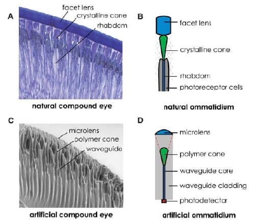
The lenses are arranged in a dome shape so that they project outwards in all directions (figure 1). This configuration provides a wide field of view similar to that of real insect eyes. The structure also helps to guide captured light into the photodetector arrays, just as the crystalline cones in nature direct light onto photoreceptor cells (figure 2).

Such eyes could eventually be used to make high-tech cameras, navigation devices in unmanned vehicles and perhaps even synthetic retinal implants. Other applications include surveillance sensors that could monitor areas over 360° and in real time. Smaller versions of such sensors could also be swallowed and be used to image inside the digestive tract, says Lee.

Nuclear waste should be buried

CoRWM was appointed in 2003 to recommend what to do with the roughly 470,000 cubic metres of waste in the UK for which there is no agreed long-term disposal strategy. This includes both existing waste and waste that will be generated over the next few decades.

The 11-strong committee, which is made up of both scientists and non scientists, is chaired by economist Gordon MacKerron. Last year, after discarding more exotic solutions such as sending the waste into space or putting it at the bottom of the sea, the panel drew up a shortlist of four options. These included two types of “geological disposal” in which the waste is buried several hundred metres underground — in either a sealed repository or one from which the waste can be retrieved for up to several hundred years after it is put in the ground. The other two options were continuous temporary storage just above or below the Earth’s surface and the burial of waste just below the surface.

The committee has now discounted the last two options, preferring instead geological disposal. But it says that this approach must be complemented by secure interim storage, pointing out that a repository might not be ready for perhaps 50 years if there are technical difficulties in developing the repository or objections from the local community.

However, CoRWM has not stated which type of geological disposal should be used. In fact, it has yet to decide whether or not it will state a preference in its final report, which it is due to release in July. It has also not said where the geological repository should be located — this was not part of its remit — but it believes that no matter where the dump is located it must have the blessing of the local residents. “The key decisions must involve potential host communities and they should have an equal footing in all relevant decision making,” says MacKerron.

The committee says that in reaching its decisions it has examined the technical, scientific, ethical and social aspects of all the potential options, having consulted over 200 technical experts and listened to thousands of members of the public and other people with an interest in the plans. But the panel has not had a smooth ride. Last year, one of its members, Keith Baverstock, was dismissed from the group and another, David Ball, walked out. Ball reportedly became disenchanted with what he saw as the panel’s emphasis of public consultation over expert advice.

Browse articles by content type

Shelf life: Simon Singh

What are the three best popular-science books?