Page 1773 – Physics World

Home » Page 1773

Composite fibres light up

Composites made of conductors, semiconductors and insulators are routinely used in electronic and optoelectronic devices. However, such devices are usually produced in elaborate wafer-based processes, which means that they are restricted to flat surfaces and small areas. In contrast, drawing fibre from a reel or tube is a much simpler technique. Moreover, it can be used to make long lengths of uniform fibres with good optical characteristics.

Yoel Fink and colleagues at MIT began by arranging a crystalline conductor (tin), an amorphous semiconductor (arsenic-selenium) and an insulator (polyetherimide) into a cylinder or “preform” about 20 centimetres long. The three components all have different refractive indices but similar melting temperatures, which means they can be processed under the same conditions.

The preform comprises a hollow air core, surrounded by a so-called omnidirectional or “perfect” dielectric mirror that is formed from eight pairs of alternating layers of arsenic-selenium and polyetherimide. Such a mirror — which was first demonstrated by Fink and co-workers in 1998 — is able to reflect light from all angles and with all polarisations, like an ordinary mirror, but it can also be tuned to only reflect at certain wavelengths.

Figure 2

Next, the MIT team heated its preform in a furnace and drew it into a thread-like fibre hundreds of metres long. This step miniaturises the macroscopic cylinder but preserves its geometry to produce feature sizes smaller than 100 nanometres. Moreover, it creates intimate contacts between the semiconductor-insulator and metal layers. The whole fibre was then surrounded with cladding made from another polymer (figure 1).

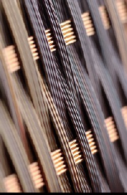
The fibres produced are able to detect light along their length and if modified — by introducing a special photoconducting glass cylinder into the core — can generate an electrical response when illuminated. When woven into a fabric with a grid structure, the device is capable of localising point sources of light (figure 2). Furthermore, the direction of incoming light could be determined if layers of the fabric were overlapped.

Fingerprint model makes an impression

Skin is made up of several layers, including the basal layer, which separates the outer epidermis and the inner dermis. Fingerprint development begins when the foetus is about ten weeks old and the basal layer begins to grow faster than either the epidermis or dermis in the tips of the finger. This leads to an increased stress in the basal layer, which causes it to buckle inwards, creating ridges on the surface of the skin. This explanation was first suggested in the 1920s by the Norwegian scientist Kristine Bonnevie but was subsequently forgotten.

Michael Kücken and Alan Newell at the University of Arizona developed a model in which the basal layer is an elastic sheet confined between the epidermis and dermis, which are modelled as beds of weakly nonlinear springs (figure 1). Due to differential growth — and the fact that it is constrained — a compressive stress builds up in the sheet that represents the basal layer. If the compressive stress is high enough, a buckling instability occurs. The scientists analysed this process by minimising the total elastic energy in their system.

Kücken and Newell say that boundary forces — produced at finger creases and nails — are the main source of stress in the fingertips of a developing foetus. They also note that stress is produced as the tips of our fingers (known as volar pads) shrink when fingerprints begin to develop. This creates ridges that are perpendicular to the direction of the stress.

Figure 2

Kücken and Newell also observed that the formation of the three basic patterns of fingerprints — known as arches, loops and whorls — is related to the geometry of the volar pads as they shrink. Previous research has shown that highly rounded volar pads produce whorls, for instance, and that flatter pads produce arches. The Arizona duo found they could reproduce these patterns in their simulations (figure 2).

They now plan to focus on the defects in the patterns that are important in fingerprint identification, including ridge endings and bifurcations.

First among equals

Some 20 equations received two or more nominations, but two very different equations were clearly considered greater than the rest — Maxwell’s equations of electromagnetism and the Euler equation. While the latter is a construction of truly bewildering beauty and simplicity, e^iπ+ 1 = 0, its relation to the physical world is not obvious.

Maxwell’s equations, on the other hand, inspired many of the great theories of the 20th century, as well as putting electricity, magnetism and optics on a solid theoretical basis for the first time. Among other things, Maxwell used his four equations — which first took shape in the 1850s and appeared in their final form in 1873 — to calculate the speed of light and predict the existence of electromagnetic waves at non-visible wavelengths.

Describing Maxwell’s equations, Heinrich Hertz once said, “One cannot escape the feeling that…they have an intelligence of their own, that they are wiser than we are, wiser even than their discoverers, that we get more out of them than was originally put into them.” And so it was that Einstein combined Maxwell’s equations with the principle of relativity to derive E = mc². And later, in 1927, Dirac applied quantum theory to them and went on to formulate his equation for the electron and lay down the foundations of quantum electrodynamics.

Maxwell’s equations also possess another subtle property — local gauge invariance — although the significance of this was not realized until Chen-Ning (Frank) Yang and Robert Mills published a ground-breaking paper on the strong force 50 years ago this month (1954 Phys. Rev. 96 191). Local gauge invariance is now known to be an essential feature of both the strong and electroweak interactions, and Yang-Mills equations are used to describe both of these forces in the Standard Model of particle physics.

In simple terms, gauge invariance or symmetry means that something — for example, the electric potential in electromagnetism — can be “re-gauged” or changed without having a noticeable effect. Local gauge invariance means that the electric potential can be changed by different amounts at different places in space and time without changing Maxwell’s equations. Indeed, some theorists speculate that the fundamental forces are nature’s way of maintaining local gauge symmetries in the world. For some reason — perhaps because it cannot be written on a T-shirt, or because gauge invariance is such a subtle concept — the Yang-Mills equation is absent from our list of great equations.

Although Hawking caused a stir when he wrote about “knowing the mind of God” at the end of A Brief History of Time, Steven Weinberg managed to escape similar controversy when he brought equations and religion together in an essay published in It Must Be Beautiful (a collection of articles about great equations that includes a chapter on the Yang-Mills equation by Christine Sutton). Weinberg compares the great equations of modern physics to cathedrals, and concludes that “they might outlast even the beautiful cathedrals of earlier ages”. Of course, as Weinberg points out, all equations in physics are approximations, but the very best will remain useful for as long as time itself.

Nanodevices target viruses

Earlier this year, the Cornell team designed a nanoelectromechanical device that is capable of weighing objects with a mass of just 10^-18 grams. The device consists of an oscillating cantilever made from a small wafer of silicon just 4 microns long and 500 nanometres wide (figure 1). When a small particle is placed on the wafer, it alters the frequency at which the wafer vibrates. This change can be measured by observing how laser light is reflected off the wafer, which then allows the mass of the particle to be calculated.

By chemically coating the cantilever with a layer of antibodies that are sensitive to a specific virus, the Cornell team has now used the same device to detect viruses (Appl. Phys. Lett. 85 2604). To do this, the cantilevers are immersed in a liquid containing the virus particles, which then stick to the device. The device is then removed from the liquid and the frequency is measured again. “The sensitivity is high,” says Craighead, “and just a few virus particles can be identified and detected rapidly.”

Figure 2

Meanwhile, Lieber’s team converted an array of nanowire-based field effect transistors (FETs) into a virus detector by coating the surfaces of the transistors with antibody receptors (Proc. Nat. Acad. Sci. 101 14017). Viruses were then introduced into arrays using microfluidic channels. Since viruses are charged particles, they change the current flowing through the transistor of the FET because they change the concentration of charge carriers when they bind to the nanowires (figure 2).

“The intrinsic amplification of the nano-transistor, and the fact that binding at the surface affects the ‘bulk’ carrier concentration, leads to extremely high single-molecule sensitivity,” says Lieber. Moreover, modifying the different nanowires within the array with receptors that are specific for different viruses allows multiple virus strains to be detected at the same time.

The Harvard researchers are developing arrays that can sense up to 100 different viruses simultaneously, and they hope to further increase the sensitivity of their technique so that it can detect single nucleic acids or proteins. The Cornell team also plans to create similar arrays.

DNA imager dies

Maurice Wilkins was born in New Zealand in 1916, the son of a doctor, and was sent to school in England at the age of six. He received a degree in physics from Cambridge University in 1938, then carried out research to improve radar screens, earning a PhD in 1940. He subsequently worked on the separation of uranium isotopes for nuclear weapons before joining the Manhattan atomic bomb project in the US.

After returning to Britain in 1945 and working as a lecturer at St Andrews University in Scotland for a year, he moved to King’s College London, where he joined the biophysics unit. He began taking X-ray diffraction images of samples of DNA and it was one such image, which he displayed at a talk in Naples in 1951, that excited a member of the audience, the young American biologist James Watson.

While Watson and Crick investigated the structure of DNA at Cambridge, Wilkins hired the crystallographer Rosalind Franklin to help him. It was one of Franklin’s X-ray diffraction images that Wilkins showed Watson and which led to Watson and Crick’s discovery in 1953 of the helical structure of DNA.

Wilkins, whose death follows that of Crick in July this year, became professor of biophysics at King’s College in 1970 and remained connected with King’s until his death. He was a prominent campaigner for nuclear disarmament and was president of the British Society for Social Responsibility in Science from 1969 to 1991. His autobiography, The Third Man of the Double Helix, was published last year.

Nanotubes shape up for spintronics

Like their carbon counterparts, nanotubes made of vanadium oxide display a variety of electronic properties depending on their detailed structure. Lia Krusin-Elbaum and co-workers at IBM’s TJ Watson Research Center in New York made multiwalled vanadium oxide nanotubes with a self-assembly technique that relied on organic molecules called amines to direct the growth of the nanotubes. The tubes produced were typically several microns long with diameters between 60 to 100 nanometres.

There were three types of vanadium atom in the structure: so-called V(2) and V(3) sites are low energy sites with relatively localized electrons which have spins that point in opposite directions. This gives rise to an overall ferromagnetic moment because there are two V(2) spins for every (V3) spin. However, the entire nanotube is non-magnetic because the itinerant electrons associated with the higher energy V(1) sites “frustrate” the magnetic order by making it impossible to form a unique ordered ground state.

Krusin-Elbaum and colleagues found that when they doped their nanotubes with extra electrons — which they did by adding lithium — the structures became magnetic (see figure). Even more surprising, the nanotubes also became magnetic when the addition of iodine removed electrons to create holes.

The team

“Removing electrons takes out enough of the V(1) electrons to eliminate their roles as spins, while lithium doping adds enough electrons to approach double occupation of the V(1) sites, which also renders them spinless,” Krusin-Elbaum told PhysicsWeb. “Hence the net result is that either kind of doping turns on ferromagnetism, in a system whose undoped state is non-magnetic.”

The team now plans to develop nanosystems in which the electron spins can be controlled by a voltage or some other physical mechanism, rather than doping.

Angular uncertainty passes test

If you asked members of the public to name a concept or idea from modern physics, the most popular answer would probably be E = mc². However, the runner-up could well be Heisenberg’s uncertainty principle. This principle states that the position and linear momentum of a particle cannot be known simultaneously with arbitrary precision. More precisely, it sets a lower bound for the product of the uncertainties of these quantities: Δ xΔp ≥ h-bar/2, where Δx is the uncertainty in the position, Δp is the uncertainty in the momentum and h-bar is Planck’s constant divided by 2π.

One consequence of the uncertainty principle is that quantum objects such as electrons do not follow classical trajectories, which is in clear conflict with our everyday experience. A similar, but less well known, uncertainty relation also exists between energy and time. Now, researchers at the universities of Glasgow and Strathclyde in the UK have studied another manifestation of the uncertainty principle. In a beautiful experiment involving light beams, the team has verified the uncertainty relation between angular position and angular momentum for the first time (S Franke-Arnold et al. 2004 New J. Phys. 6 103).

Uncertain world

The angular position of a particle, Φ is simply the angle at which it is located in 2D “polar” co-ordinates. The angular momentum, L, is the rate of change of this angle with time multiplied by the mass of the particle and the square of its polar radius. A light beam consists of many photons, each of which has an angular position and an angular momentum, so the beam is best described by a probability distribution of angles. The uncertainty in the angular position, ΔΦ, is the typical spread of the angles among the photons.

In its general form, the uncertainty principle applies to every pair of “conjugate” variables (in quantum mechanics two variables, A and B, are said to be conjugate if AB – BA = ih-bar). It might therefore seem that the uncertainty relation between angular position and angular momentum is exactly the same as that between linear position and momentum. But things are not quite this simple because the angular position is restricted to values between -π and +π, whereas linear position can take any value. This has two interesting consequences. First, the uncertainty in the angular position is always finite. Second, the angular momentum is quantized and can only have certain values known as eigenvalues, whereas linear momentum, like linear position, can take any value. When the angular momentum assumes only one of these eigenvalues, the system is said to be in an angular-momentum eigenstate.

Since the uncertainty in the angular momentum, ΔL, is zero for any angular-momentum eigenstate, the product of ΔΦ and ΔL is also zero. It therefore seems as if these two conjugate variables can beat the uncertainty relation. However, when a system is in an angular-momentum eigenstate, we know absolutely nothing about its angular position. Conversely, if the angular position is confined to a narrow range of values, then the angular momentum must be distributed over a broad range of values (i.e. the system must be in a superposition of many different angular-momentum eigenstates). Mathematically, this is expressed as ΔΦΔL ≥ (h-bar/2)[1 – 2πP(π)], where P(π) is the probability that the angular position has a value of π.

It is natural to ask, which states satisfy the equality in this relation? Sonja Franke-Arnold and Stephen Barnett at Strathclyde have now calculated that the only distribution of angular position that satisfies this “minimum uncertainty” state is a Gaussian that is truncated at ±π. When the uncertainty in Φ is large, the probability of obtaining one eigenvalue of L is large and the probability for all other eigenvalues of L is small. In this case, the product of the two uncertainties is small. Conversely, for small uncertainties in angular position, the distribution of Φ is narrow and P(π) is small. Here, the angular-momentum distribution is broad and closely resembles a normal Gaussian. This situation is reminiscent of the normal position-momentum uncertainty relation, and the value of the uncertainty product ΔΦΔL is indeed close to h-bar/2.

Experimental certainty

Guided by the Strathclyde group’s theoretical work, Eric Yao and colleagues at Glasgow prepared a beam in which the angular position followed a Gaussian distribution, and then measured the resulting distribution of angular momentum. To do this, they inserted an absorber in the path of a broad light beam that let different amounts of light through depending on the light’s angular position. The absorber has a wedge shape that looks like a cake slice, and it imprints the desired angular distribution onto the intensity profile of the beam. The easiest way to make such a spatial light absorber is to use an array of liquid-crystal pixels that can be programmed with a computer. Diffraction from the absorber changes the angular-momentum distribution.

The angular momentum can then be measured using an appropriate holographic grating followed by a lens and a pinhole (the light intensity passing through the pinhole indicates the probability of finding a specific eigenvalue of the angular momentum). For a series of absorbers with different uncertainties in angular position, the observed angular-momentum distributions agree well with theory and are consistent with the uncertainty relation derived by the Strathclyde group.

This work beautifully illustrates that uncertainty relations for quantities other than position and momentum are not just theoretical constructs but can also be explored in the lab. The Glasgow experiment illustrates this uncertainty relation for the wave nature of light, which can be fully described by classical electrodynamics. But a lot of the relevant quantum physics is already captured in the present set-up because the wave description of light and the de Broglie picture are similar. The Glasgow group is now repeating the experiment for single photons, in order to investigate the angular-uncertainty relation for a genuine quantum system.

Hunting cosmic explosions

There is a Persian fairytale about the three princes of Serendip — the island in the Indian Ocean that is now known as Sri Lanka. The princes were seasoned travellers who made a series of astonishing discoveries through good fortune alone. Their luck was so amazing that we now use the word “serendipity” to describe what happens when we find something unexpectedly. As the discovery of gamma-ray bursts makes clear, serendipity often plays a key role in science.

The story began in 1963 when the world’s leading nations signed the nuclear test-ban treaty, which sought to prevent nuclear bombs from being exploded underwater or above ground. That year the US also launched the first of a series of satellites called the Velas — named after the Spanish for “watchmen” — that were designed to monitor radiation from clandestine nuclear explosions. Like the legendary princes of Serendip, the Velas made an unexpected discovery.

On 2 July 1967 one of the satellites detected a sudden bright flash of gamma rays. It then saw another from a different direction, and then another. These unexpected flashes kept coming, outshining everything else at gamma-ray frequencies for several minutes. It soon became apparent that these bursts of light were not from man-made sources and that they did not originate from the Earth, the Sun or even any of the planets.

It was not until 1973, however, that Ray Klebesadel, Ian Strong and Roy Olson of the Los Alamos National Laboratory in the US announced the discovery of what they called “gamma-ray bursts”. They waited so long to reveal their findings because they wanted to be sure that the flashes of light came from somewhere in space. Contrary to popular mythology, security considerations played no role in the delay before the findings were made public.

Figure 1

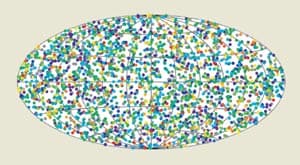
In the years that followed, theorists applied their minds to the mystery of these bursts, and a number of imaginative solutions were proposed. However, a lack of key observational data meant that real progress in the field only began in 1991 when NASA launched the Burst and Transient Source Experiment (BATSE) on board the Compton Gamma-Ray Observatory. Over the next 10 years it detected over 2700 gamma-ray bursts, distributed evenly across the sky (figure 1). Gamma-ray bursts clearly had nothing to do with any objects in the solar system, the Milky Way or any known nearby galaxies, otherwise they would be clustered only around certain directions.

Astronomers realized that the bursts must be caused by some sort of dramatic event — possibly an explosion. To find out more, they naturally turned to ground-based telescopes to search for possible “afterglows” of these events at optical and other wavelengths. This radiation, they reasoned, might give clues to the origin of the bursts.

Unfortunately, BATSE could not pin down the location of a gamma-ray burst to much better than 1 or 2 degrees. Such large regions of the sky — which are several times the diameter of the Moon as seen from the Earth — contain vast numbers of other objects that also emit visible light. Astronomers therefore did not know where precisely to point their telescopes to find out more about bursts that had been spotted by BATSE. Progress stalled.

Burst breakthrough

While observers were trying to detect the afterglow of gamma-ray bursts, Peter Mészáros of Penn State University in the US and Martin Rees of Cambridge University in the UK published a seminal paper in 1993 that predicted how an afterglow could be created (see further reading). They argued that any sort of explosion depositing a large amount of energy in a small amount of matter would invariably lead to a fireball travelling at very near the speed of light. This powerful jet would sweep up matter from its surroundings. Any electrons that were present would be accelerated, causing them to emit synchrotron radiation — the afterglow — at all wavelengths. Mészáros and Rees’s theory also predicted that the afterglows would fade rapidly at first and then more gradually — in other words, the radiation would follow a power law. The bursts might therefore last long enough to be observed (see Physics World April 1997 p10 and June 1997 pp23 to 24).

The breakthrough came on 28 February 1997 — almost 30 years after the first gamma-ray burst was detected — when astronomers pointed the Italian-Dutch BeppoSAX satellite in the direction of a burst that had occurred just eight hours earlier. They hoped that the on-board detectors would see a fading X-ray signal — the dying embers of the gamma-ray burst — at the very same point in the sky where the burst had been observed. Remarkably, they succeeded. This was the first direct observation of the afterglow of a gamma-ray burst and it sparked a revolution in research into these cosmic explosions.

Soon afterwards, gamma-ray-burst afterglows were found to emit not just X-rays and gamma-rays but radiation across the entire electromagnetic spectrum. However, it took another six years to establish the nature of these elusive sources. We now believe that gamma-ray bursts are the most energetic explosions that stars ever experience — even more powerful than supernovae — and that they can be seen from the Earth across the entire volume of the visible universe.

Hunting down gamma-ray bursts

If you look at the night sky with a powerful optical telescope, you will find that it is lit with millions of dots. You would have a very hard time trying to pick out gamma-ray bursts among all these other objects. Most astronomers therefore search for the bursts at gamma-ray wavelengths, where such sources are few and far between. Following the retirement of BeppoSAX in 2002, most gamma-ray bursts are currently detected by the US’s High-Energy Transient Explorer (HETE-2) and Europe’s International Gamma Ray Astrophysics Laboratory (INTEGRAL).

However, astronomers have to act quickly because gamma-ray bursts fade relatively fast. Once a burst has been roughly located to arc-minute accuracy with one of these satellites, its position is immediately distributed to astronomers and observatories around the world via the Gamma-Ray Burst Coordinates Network (GCN). The burst is then pinned down to arc-second accuracy either at X-ray wavelengths using the Chandra X-ray Observatory or the XMM-Newton satellite, or using ground-based optical or radio telescopes, such as the Very Large Array (VLA) in New Mexico.

Figure 2

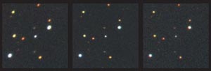
Astronomers know that they have tracked down an afterglow when they find a previously unknown source with an intensity that decays with time (figure 2). They can then carry out detailed studies of the light from the burst using spectrographs or optical CCD cameras. The afterglow usually lasts for days to weeks at optical and X-ray frequencies — and months in the case of radio waves. Observers therefore have some time — although not much — to obtain good-quality optical spectra.

These spectra often have absorption lines, which indicates that certain wavelengths have been absorbed by matter as the radiation travels from the source of the burst to the Earth. By measuring how much these lines have been red-shifted to longer wavelengths as a result of the expansion of the universe, astronomers can determine how far away the burst is. The immediate and irrefutable result of this work is that gamma-ray bursts originate in galaxies at cosmological distances — sometimes even near the edge of the observable universe. The most distant burst ever detected was spotted on 31 January 2000 by Michael Andersen of the University of Oulu in Finland and his colleagues at the University of Copenhagen, including one of us (JH). Its light was emitted when the universe was just 1.4 billion years old — 10% of its current age.

Gamma-ray bursts are so distant and have such high fluxes of radiation that their total energy output is huge. For example, gamma-ray burst 990123, which was seen on 23 January 1999, was initially believed to have released about 4 x 10⁴⁷ J of energy — more than would be generated if the entire mass of the Sun or a neutron star were converted into gamma rays. This figure seems absurdly high, because we know of no credible mechanism that could convert such a huge mass into gamma rays in a matter of seconds. However, gamma-ray bursts do not emit equal amounts of energy in all directions, as astronomers had previously assumed. If the radiation is emitted from just a very small part of the fireball (like a lighthouse beam) a quick recalculation reduces its total energy by a factor of 100-1000. The energy output is now in the realm of the believable — typically 10⁴⁴ to 10⁴⁵ J — which is not much more than that of a supernova.

Astronomers soon gained corroborative evidence that the outflow from a gamma-ray burst is collimated in this way. The most compelling evidence came when they found that the afterglow starts to fade more quickly with time, which hinted at changes in the geometry of the emitting regions. What seems to be happening is that the jet that produces the afterglow expands as it slams into matter that surrounds the source. It therefore slows down and beams its radiation to a larger angle. The beam becomes less collimated as it expands, causing the afterglow to start to fade more rapidly. This sudden drop, or break, in the afterglow light curve occurs at all wavelengths and can be used to calculate the angle of the initial cone of radiation and hence the total energy released at the source.

But if we are only observing emissions from a narrow cone that happens to be in our line of sight, then surely there must be hundreds of other gamma-ray bursts that we cannot see because they shine in other directions. So how often do they really occur in the universe? The jury is still out on this question, but the true number is probably hundreds — and possibly even thousands — per day in the observable universe.

The supernova connection: a one-two punch

In 1993 one of the present authors (SW) wondered if gamma-ray bursts are linked to supernovae — bright explosions that occur during the death-throes of stars that are at least eight times more massive than the Sun. When such stars deplete their nuclear fuel, they no longer have enough energy and pressure to support their mass. The core implodes, forming either a neutron star or — if there is enough mass — a black hole. The energy released by this collapse flings the surface layers of the star outwards, creating a bright explosion. Although most supernovae cannot produce gamma-ray bursts because their explosion velocities are too slow to make gamma rays, a special type of supernova — in which most of the energy is transferred to jet-like outflows along the rotation axis — could produce the fireballs that are believed to create gamma-ray bursts.

True to the call, an unusually energetic supernova was detected in late April 1998, named SN1998bw. It appeared to be near a gamma-ray burst that had occurred just a few days earlier on 25 April. Astronomers argued that the probability of this happening by chance was less than 0.01%. SN1998bw appeared to provide tantalizing evidence for a possible link between supernovae and gamma-ray bursts. But could the researchers really be sure? Many astronomers were sceptical. This particular gamma-ray burst, they argued, was an odd one, being several orders of magnitude less energetic than common gamma-ray bursts. The supernova itself was also unusual, they said.

It was not until last year that we could confidently say that we had found the “smoking gun”. On 29 March 2003 the HETE-2 satellite observed, in the constellation Leo, one of the brightest and closest gamma-ray bursts on record. Ground-based follow-up observations of its afterglow revealed, for the first time, that a gamma-ray burst and a supernova had occurred essentially simultaneously — a quick and powerful one-two punch. GRB 030329 occurred only two billion light-years away (Physics World May 2003 p3). The burst lasted about 30 s and it was among the top 10 brightest bursts ever recorded to date. Its afterglow lingered for weeks at lower-energy X-ray, radio and visible wavelengths.

However, only direct observational evidence would prove once and for all that gamma-ray bursts and supernovae are linked. Working with members of the international Gamma-ray Burst Afterglow Collaboration at ESO (GRACE), the present authors decided to monitor the afterglow to see if we could detect the characteristic spectral features of a supernova in the fading light of the burst. (A competing group

led by Peter Garnavich of the University of Notre Dame and Thomas Matheson and Kris Stanek from the Harvard-Smithsonian Center for Astrophysics also carried out the same test.) Within days, we had discovered broad lines in the optical afterglow that were very similar to those seen in the spectrum of supernova SN1998bw. These lines indicated that we were witnessing a massive, rapidly expanding supernova shell, sometimes called a “hypernova”, that was moving as fast as 12% of the speed of light. Projecting these expansion velocities back in time, we concluded that the supernova of 29 March 2003 had indeed exploded at the same time as GRB 030329. The link between supernovae and gamma-ray bursts was proven.

The gamma-ray burst that took place on 29 March 2003 changed everything for researchers in the field. Astronomers are now sure that at least some gamma-ray bursts are produced when black holes — or perhaps very unusual neutron stars — are born inside massive stars. Gamma-ray bursts are so bright that, during the fleeting moments of their existence, they emit as much energy as 10 million billion Suns.

Figure 3

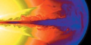
But what exactly happens during this process? Although Mészáros and Rees’s fireball model is still the most popular explanation of the essential physics of the afterglow, it and other competing models deal with the aftermath of these explosions. The best contender for how such a fireball is created in the first place is known as the “collapsar” model, which was first developed by one of us (SW) back in 1993 and explored further with Andrew MacFadyen, who is now at the California Institute of Technology (figure 3).

How gamma-ray bursts are made

The story starts hundreds of thousands of years before the explosion that creates the gamma-ray burst when a massive gaseous star runs out of fuel and sheds its outer envelope of hydrogen and helium. Driven off by the star’s own radiation, or perhaps lost to a binary companion star, the loss of the envelope turns the star into a bluish compact star. The remaining star — containing about 15 solar masses worth of helium, oxygen and heavier elements — quickly loses its remaining fuel and its inner core collapses to form a black hole. At the same time, parts of the star pile up in orbit around the black hole to form an accretion disk, while the outer layers of the star respond more slowly, unaware of the catastrophe in progress at its heart. Powerful electric and magnetic fields are generated because the inner part of the disk rotates much faster than the edge, perhaps amplified by the rapid rotation of the black hole itself.

These fields launch jets of matter that flow out along the rotational axis of the star. They burrow with ease through the outer parts of the star, taking about 10 s to get there. Meanwhile, winds of super-hot neutrons and protons blow away from the disk. As the winds cool, these particles reassemble to form tightly bound nuclei such as nickel-56. The winds and the jets shatter the star in a gigantic explosion — a supernova. About an hour later, far outside the original star, collisions occur between pieces of jet that are moving at different velocities near the speed of light . These collisions are responsible for the gamma-ray burst, flinging radiation in our direction. Days and weeks later, the nickel-56 decays into cobalt-56 and iron-56, producing the energy that makes the supernova shine so bright.

X-ray flashes

If the outflow from a collapsar is indeed collimated, then perhaps just one in every few hundred of the ensuing jets will be aimed at the Earth. Could it be that there are many more explosions that we have not yet seen, caused by jets that are not pointing at us? If so, what would they look like?

The collapsar model provides the answer. We now know that the matter in the jets of a gamma-ray burst is ultra-relativistic — in other words, it is moving at about 99.999% of the speed of light. Depending on the angular structure of the jet, off-axis emissions are produced by somewhat more slowly moving matter. This material will be less affected by the Doppler effect and its intensity will therefore peak at a lower frequency (and hence lower energy) than the on-axis emissions.

So if we want to spot gamma-ray bursts caused by off-axis emissions, we should look at X-ray frequencies. Remarkably, nature complied. Shortly before the BeppoSAX satellite retired, it discovered brief flashes of X-rays that had very little accompanying energy in the gamma-ray regime. These flashes have since been confirmed by the HETE-2 satellite. Could these X-ray flashes be gamma-ray bursts seen slightly off-axis?

To find the answer, we need to consider what fingerprints these flashes would leave on our data. First, we can expect the afterglow to be invisible initially, since it points away from us. It will then come into sight as the outflow slows down, before decaying like the afterglow from any other burst. Second, if X-ray flashes and gamma-ray bursts are two manifestations of the same physical phenomenon, and if gamma-ray bursts are associated with supernovae, then X-ray flashes should also be accompanied by supernovae. The third clue comes from the fact that off-axis emissions are less intense than head-on gamma-ray emissions: we will therefore tend to spot only those X-ray flashes that are particularly bright — and hence closer — than conventional gamma-ray bursts. Finally, we can expect to detect more X-ray flashes than gamma-ray bursts.

All of these properties were exhibited by an X-ray flash that was observed by detectors on-board the HETE-2 satellite on 23 July 2003. Its optical afterglow was found by Derek Fox and colleagues at Caltech using the Palomar 60 inch telescope. Its light curve was measured by Johan Fynbo and colleagues at the Niels Bohr Institute in Copenhagen, working with members of the GRACE collaboration (figure 4). More and more phenomena are now being tied together in the overall picture of gamma-ray bursts and it is becoming clear that the bursts are a motley crew of explosions transcending the gamma-ray astronomy field.

Figure 4

Swift progress expected

Although there has been great progress in our understanding of gamma-ray bursts over the last few years, the mystery has still not yet been fully solved. New light could be shed on the puzzle by a NASA-led international satellite named Swift, which will be launched this month (see news story on page 12 print edition only). It will be able to locate gamma-ray bursts within seconds of them being observed. Once an event triggers an on-board telescope, the satellite will automatically and “swiftly” repoint its own X-ray, optical and ultraviolet instruments at it. With the mission likely to pinpoint as many as 100 bursts every year, afterglow hunters will be busier than ever.

One of Swift’s aims is to study a type of gamma-ray burst that was first observed by one of us (CK) and her colleagues at NASA’s Marshall Space Flight Centre in Huntsville, Alabama, using BATSE in 1993. This team found that some gamma-ray bursts last for no more than 2 s and contain relatively large number of photons at high energies. These “short” bursts are very different from the more familiar “long” bursts. About a quarter of gamma-ray bursts are of the short variety, but none of them has been accurately located, leaving the question of where they come from unanswered. We do not know if they are associated with the deaths of massive stars — or even with galaxies. Are they a variant of collapsars or perhaps merging neutron stars? A crucial test will be to look for afterglows as well as possible supernova signatures in their afterglows.

Thanks to its highly sensitive instruments and large field of view, Swift will also be able to detect many more faint gamma-ray bursts — both on- and off-axis — than previous satellites. Some of these bursts will be intrinsically faint, but some will be dim because they are simply very far away. These bursts will therefore be extremely important tracers of star formation, enabling astronomers to probe the physical conditions of the universe when the first stars were forming (see “Star formation” on pages 25 to 29 print edition only). Gamma-ray bursts could therefore tell us not only about how massive stars died, but also how they were born.

As an added bonus for those who get their thrills from stellar explosions, Swift will also be a splendid supernova hunting machine, given that we now know that the two phenomena are inextricably linked. In particular, it will be able to detect a significant population of intrinsically faint bursts at modest distances. As these are more likely to be off-axis than on-axis, the supernova will not be hidden by the bright afterglow of the burst. It should therefore be easy to study how supernovae evolve in the first few minutes, days and months after the burst. Swift will also let us study supernova explosions very soon after they occur and detect many more Type Ic supernovae, providing an unprecedented insight into the geometry of supernova explosions.

Swift promises to herald the start of a fascinating new era of research.

The top quark: an unbiased tale

In the world of high-energy physics, experimental teams publishing the results of a search for some new phenomenon — let’s call it a snark — usually telegraph the results via a code word in the title of the paper. If the statistical significance for the snark is weak or non-existent, the title of the paper will contain the words “Search for the snark…” or “Limits on snark properties…”. If, however, the statistical significance is beyond reproach, the paper might be called “Observation of the snark?” or, more dramatically, “Discovery of the snark…”.

But there is a nether world where the statistical significance for the snark might be too strong to ignore but too weak to claim a discovery. It is precisely this situation in which the CDF collaboration at Fermilab, near Chicago, found itself in late 1993. The 500 or so physicists in the team were searching for the top quark — the sixth and presumably last fundamental constituent of the Standard Model of particle physics. The result of their efforts was a mammoth 61-page paper in the journal Physical Review D (50 2966) with the unwieldy title, “Evidence for top quark production in p-bar-p collisions at √s = 1.8 TeV”. The word “evidence” was chosen carefully.

This book by Kent Staley tells the story of how the discovery was made. Staley is a philosopher at St Louis University who became interested in the top quark when he was a graduate student at Johns Hopkins University. While carrying out research for his PhD, Staley petitioned for — and was given — unprecedented access to the inner workings of the CDF collaboration, including unpublished internal documents and extensive interviews with some of the participants.

Out of this voluminous raw material of how “big science” is really done, Staley has produced a remarkable book, or, more correctly, two books pressed into a single volume. The first (and in my opinion more successful) is a rollicking good story that emphasizes the human side of an important scientific enterprise — the exhilarations and frustrations of the principal characters, the heated debates within the collaboration, and finally the tedious consensus-building required to produce the published paper. The second part is addressed to Staley’s fellow philosophers of science. It uses the CDF paper as a vehicle for considering epistemological questions, such as the nature of statistical evidence, the role of biases and subjective opinions versus objective reality.

The book begins by describing how the top quark first appeared in the Standard Model. Unfortunately, Staley then wanders off in a detour on the state of theoretical physics in pre-war Japan, how it was perceived in the West, and when or whether proper credit was given to its authors. While some interesting philosophical and historical questions are raised — including never before published details on the recognition of Kobayashi and Masakawa’s work — this material is at best peripheral to the aim of the book. It would have benefited from either more severe editing or being spun off into a separate monograph.

Staley fares much better in his introductory material on the history of the CDF detector and collaboration. There is a good balance between his descriptions of the detector and his explanations of why it was built. This section includes various social and political aspects of the detector’s construction, the lab’s competition with CERN, and the exigencies of funding and schedules. Staley is correct in emphasizing that the design of the detector was driven by a philosophy that the instrument should extract the most (and most precise) information per event — rather than be narrowly optimized for any particular physics signature, even for the top quark. The result was a general-purpose device that adapted gracefully to changing physics interests and requirements.

Staley is most readable in the middle part of the book, where he follows the struggle within the CDF collaboration while the participants debated the strengths and weaknesses of their statistical (and other) evidence for the top quark. As he writes, “Big science presents a big opportunity for methodologists. With their constant meetings and exchanges of e-mail, collaboration scientists routinely put their reasoning on public display, long before they write up their results for publication in a journal.”

I was particularly interested in Staley’s examination of possible bias in the methodology and how the CDF collaboration dealt with it. When particle physicists try to find a particular set of events among the trillions of collisions that occur in an accelerator, they have to focus their search by ignoring data outside a certain range. In the case of the top quark, the CDF physicists knew that they could select their data in two different ways. Although both approaches were valid, the one they chose turned out to produce a stronger signal. Clearly, there is a danger in admitting a non-physicist to such raw material, since a lack of understanding of the issues and conventions can easily lead to very wrong, even silly, conclusions. I am impressed that Staley “got it right”.

At the end of the book, Staley changes from reporter to philosopher. He realizes that the CDF’s methodology does not fit neatly into any conventional models of the history of science. Instead, he offers his own theory of “error-statistical evidence”. I found this section tough going, replete as it is with ponderous sentences like, “The distinction between the epistemic and causal relevance of epistemic states of experimenters may also help to clarify the debate over the meaning of the likelihood principle.”

On the other hand, I did appreciate some of Staley’s humorous examples to illustrate abstruse constructions. Here I freely admit that Staley is a better physicist than I am a philosopher. As evidence of my incompetence, I had to look up the meaning of ceteris paribus (other things being equal). And just as Voltaire’s Monsieur Jourdain was surprised to learn that he had been speaking prose all his life, so I was intrigued to find that I had been practising “Neyman-Pearson hypothesis testing” during my time on the collaboration.

Ultimately, scientific research and discovery is a very human enterprise from solitary author to large collaborations. Personalities, ambitions and communication skills do affect the exact course that scientific enquiry takes in approaching a better approximation to the laws of nature. As a philosopher, Staley is comfortable in embracing this condition, and he makes a good case for the self-correcting nature of the process and the ultimate objectivity of the result.

Strong-force theorists scoop Nobel prize

The strong force is what binds quarks together inside protons and neutrons in an atomic nucleus. The discovery made by Gross, Politzer and Wilczek implied that when quarks are very close to each other, the force between them is so weak that they behave almost as free particles. Conversely, when the quarks move apart, the force becomes stronger as their separation increases. This phenomenon is called asymptotic freedom and it explains why quarks cannot normally be removed from an atomic nucleus.

This discovery was expressed in 1973 in a mathematical framework that laid the foundations for the new theory of quantum chromodynamics (QCD), which describes the strong force. The theory was an important contribution to the Standard Model of particle physics, which also describes the weak and electromagnetic forces. With the aid of QCD, theorists can explain why quarks only behave as free particles at extremely high energies. QCD has been tested in detail in recent years, in particular at CERN in Geneva.

The discovery was originally published in two back-to-back papers in Physical Review Letters — one by Gross and Wilczek and the other by Politzer. Wilczek and Politzer were only graduate students at the time. The prize, which is worth 10 million Swedish kroner, will be shared equally between the three laureates.

Browse articles by content type

Composite fibres light up

Fingerprint model makes an impression

First among equals

Nanodevices target viruses

DNA imager dies

Nanotubes shape up for spintronics

Angular uncertainty passes test

Hunting cosmic explosions

The top quark: an unbiased tale

Strong-force theorists scoop Nobel prize

Physics World Weekly

Physics World Stories

Reset your password

Registration complete