The Chancellor of the Exchequer, Gordon Brown, made the announcement as part of his presentation of the government’s biennial spending review. He said that science funding will rise from £3.9bn in 2004/5 to £5bn in 2007/8, amounting to an average growth in real terms of 5.8% per year. This will provide central funding for research councils so that they can “respond more quickly to emerging priorities and opportunities”, and will give universities more money to spend on improving their crumbling labs. It will also provide additional money for researchers to commercialize their research and more support for businesses to ensure they make the best use of university research.
The ten-year plan sets out the government’s aim for increasing public and private spending on R&D between now and 2014. It includes a number of measures to improve science education, including more pay for some teachers and the introduction of at least one teaching assistant for science subjects in every secondary school in England. It also increases teacher-training bursaries for science graduates to £7000 and boosts “Golden Hellos” for new science teachers to £5000.
Julia King, chief executive of the Institute of Physics, says the Institute welcomes the extra science funding but believes that the government must address a number of issues affecting the supply of physicists, particularly education. “The first step is to invest in the infrastructure of school science teaching and university physics departments, and to foster a community in Britain that is welcoming to science,” says King.
Details of how the new money will be divided up between disciplines will be announced later this year.
Kirkby and colleagues have presented new data on the cosmic-ray flux as recorded in the beryllium-10 content of deep ocean sediments. They say that the data suggests a link between the number of cosmic rays arriving on Earth and the glacial cycles. Beryllium-10 is produced when cosmic rays interact with particles in the Earth’s atmosphere and then falls to the ground, where it is stored in ice or ocean sediments.
The possible links between cosmic rays and glacial cycles follows on from previous work that linked cosmic rays to climate change. In 1997 Henrik Svensmark and Eigil Friss-Christensen of the Danish Space Research Institute proposed that high fluxes of cosmic rays could lead to more clouds and a cooler climate, and vice versa. The Danish scientists proposed that changes in the strength of the solar wind — the stream of charged particles that flows from the Sun — could lead to changes in the cosmic ray flux.
Kirkby and co-workers have now put forward two new mechanisms that could cause the cosmic ray flux to vary. One is an orbital modulation of the geodynamo that would results in changes in the strength and direction of the Earth’s magnetic field. Such an effect was recently discovered in long-term measurements of the geomagnetic field and can also, say Kirkby and co-workers, be seen in the beryllium-10 data. Measurements on stalagmites in northern Oman and the Austrian Alps provide further support for this hypothesis.
“The idea suggested is controversial but not crazy,” says Peter Thejll of the Danish Meteorological Institute. “I think it is well worth discussing.”
The standard insolation model of glacial cycles was first put forward by the Serbian astrophysicist Milutin Milankovitch in 1912. Milankovitch proposed that ice ages were caused by variations in the amount of sunlight hitting the Earth and were linked to a very gradual cyclic change in the shape of the Earth’s orbit around the Sun. However, while the insolation model can explain a glacial cycle with a period of the 41 kiloyears (kyr) that is observed in the paleoclimatic data, it predicts a 400 kyr cycle that has not been observed. Moreover, it cannot explain a 100 kyr cycle that is also present.
Frederick Lindemann was an exceptional person who achieved a position of influence in both the scientific and political worlds.He was born in Devon in 1886 into a reasonably wealthy family. His mother was American and his father was German, and at the age of 14 Lindemann was sent to Germany to be educated, where in due course he obtained his doctorate from the University of Berlin.
In 1919, aged just 33, Lindemann was appointed Dr Lees Professor of Experimental Philosophy and head of the Clarendon Laboratory at Oxford University. He immediately set about rebuilding the lab’s research, appointing staff from elsewhere in Britain and arranging for Francis Simon and later Nicholas Kurti, Kurt Mendelssohn, Heinrich Kuhn, and Heinz and Fritz London to leave Germany and come to Oxford.
Lindemann was a close friend of Winston Churchill, visiting him frequently and also strongly supporting his campaign for rearmament in the 1930s. When Churchill became a member of the government in 1939 and Prime Minister the following year, Lindemann became his scientific advisor. This role, however, steadily expanded to include giving advice on economics and other matters. In 1941 he became a member of the House of Lords (as Lord Cherwell) and joined the cabinet as Paymaster-General.
Prof by Adrian Fort is a very enjoyable read because it describes the complex and varied career of this distinguished but little known man. The book reveals the many contradictions in Lindemann’s character. He spent 13 undoubtedly happy years in Germany, carrying out physics research and enjoying his social life. Yet later he became a fervent supporter of Churchill in his campaign against appeasement.
Fort faithfully captures these contradictions and explains them and their ramifications through the life of Lindemann. As a physicist, I would have liked to have read more about his science in Germany and at Oxford, but what we are told is largely correct — a considerable tribute to a non-scientist writing about the origins of quantum mechanics. There is also comparatively little about the changes in the Clarendon Laboratory that Lindemann helped bring about.
The world has now changed and we are all experts in our narrow fields of interest. It is unlikely that a professor of experimental philosophy (physics) will again become an expert in economics, Paymaster-General and a member of the cabinet. This book is a very enjoyable account of a little studied but enormously interesting man, and it deserves to be read widely.
In the July issue of Physics WorldRoger Cowley, Dr Lees Professor of Experimental Philosophy at Oxford University, reviews this book in full.
Can the behaviour of people be quantitatively determined, either using equations or computers? That is the question that science writer Philip Ball tackles in his latest book. Although it is relatively difficult to predict the actions of an individual person, Ball shows – using a variety of examples – how the collective behaviour of groups of people can be reliably described using various approaches borrowed from statistical physics. I very much agree with the author, whose book provides a timely survey of the latest developments at the interface between physics and the social sciences.
Originally developed to describe the behaviour of zillions of interacting molecules, it is perhaps surprising that statistical physics is relevant to social situations. But to show how it can be applied to, say, crowd behaviour, consider the following thought experiment. Imagine thousands of people standing in a public square, all of whom are asked to turn and look in one – previously undetermined – direction. If they all manage to face in the same direction, they would be demonstrating what is called “collective behaviour”.
But in practice would the entire crowd actually look in the same direction? Statistical physicists would say that it cannot be done. They would point to the theory of particles with short-ranged ferromagnetic interactions, which states that, for a 2D system in which the magnetic particles can continuously change direction, no long-range ordered phase can exist at finite temperature and zero external field. In other words, the particles will not point in the same direction. The same, by extension, should be true for people standing on a surface, which is just another 2D system.
So what does the crowd do? Locally, everyone will look in roughly the same direction. But on a large scale – when viewed from, say, a helicopter – people form vortex-like directional patterns. These are caused by slight perturbations in the directions in which people look, as a result of human error. Curiously, however, if the members of the crowd are told that they can choose to look in one of a few, given directions, the ordering can be realized. In other words, the whole crowd will look in the same direction, if given a choice of where to look! I first described this unusual analogy with ferromagnetic systems in 2001 in an essay in Nature on collective behaviour (411 421).
Perhaps even more interestingly, the models of collective motion described in the book predict that if people are asked to move in the same, previously undefined direction they will actually move in that direction. Motion produces an effective interaction, the range of which grows with time and causes global ordering. Something similar can be seen every year when thousands of Muslims circle in a well organized pattern around the Kaba stone in Mecca during Hadj as they try to avoid colliding with each other.
Ball discusses a range of behaviour – from the intricate patterns of colonies of bacteria to the complex structure of the World Wide Web. What unites these diverse phenomena is that they all take place in systems consisting of many similar units that interact in a relatively well defined manner. These interactions can be simple (attractive or repulsive) or more complex (combinations of simple interactions) and may take place between neighbours in space or on a specific underlying network.
Under some conditions, various transitions occur in such systems. During such transitions, these objects – be they particles, organisms, people or even robots – behave in a way that is almost totally determined by the collective effects of every other object in the system. The universality of these transitions follows from a celebrated theoretical framework in statistical physics called the “renormalization group method”, for which Kenneth Wilson received the 1982 Nobel Prize for Physics.
Ball displays a good understanding of the many different theoretical approaches to the “physics of society” and seems to know many of the researchers at the forefront of this research. He also provides a vivid and entertaining account of the historical background to the field. I particularly enjoyed reading about the various scholars who had been thinking about these topics several hundred years ago. In 1690, for example, the English anatomist and political thinker Sir William Petty considered the possibility of “political arithmetick” and calculated – using only numbers and simple assumptions – that “the King of England’s Subjects, have Stock, competent, and convenient to drive the Trade of the whole Commercial World”.
I was amazed to learn that there was also a flow of knowledge from the social sciences to physics. For example, when trying to understand the role of fluctuations in the world of atoms, James Clerk Maxwell was greatly inspired by the observations of social scientists like Henry Thomas Buckle. In the 1850s Buckle was one of the first historians to appreciate the role of statistics in understanding the behaviour of large numbers of quite different individuals. Could it be that Karl Marx – who wanted to describe societies with fundamental laws – also used analogies with non-living matter when constructing his theory of economics?
After providing the necessary historical and scientific background, Ball takes the reader on a long journey from the simplest forms of collective behaviour (such as people moving together) to complex situations such as the stock market or the Internet. He introduces many of the approaches that let us interpret social phenomena in quantitative terms. For example, the behaviour of people who buy stocks and shares can be modelled by many interacting “agents”. These can be represented by an algorithm that is tuned to make rational moves depending on the actions of the others.
Other models, meanwhile, examine how collective decisions are arrived at. What, for example, determines how people vote for different political parties? How can fashion, views or people be influenced? What is the “critical mass” needed to make, say, a haircut fashionable or to excite or calm rioters? Some simple models have been built to address these questions; their success depends on the complexity of the situation.
Perhaps the most successful approach has been to interpret how people interact in terms of a “hierarchical” network. It turns out that the number of “links” we have – be they friends or e-mail, business or sexual partners – is extremely unevenly distributed. Most of us have relatively few links, but there is a small number of people who have many. This finding has led to a better understanding of how infections spread in society.
In an age when we are all cleverly manipulated by the power of advertising, big business and politics – when it is hard to judge what is “real” and what is apparent in a society – it is reassuring to know that there are fundamental scientific laws behind some of our group behaviour. I highly recommend this book to anyone who prefers to rely on firm quantitative approaches, rather than mere speculation, when trying to understand the life that surrounds them.
• Philip Ball’s article “Utopia theory” appeared in Physics World last year (October 2003 pp29-33)
Nowhere is the relevance of physics to everyday life more obvious than with the success of the DVD in the home-entertainment market. Sales of DVD players and recorders are booming, and last year consumers around the world spent over $20bn on DVD disks. In the UK, for instance, sales of DVD disks were more than twice those of video cassettes.
While physicists might sometimes complain about the “bad physics” in the movies that people watch on DVD, when making a case for the importance of their subject they should also stress that the relentless march of the DVD into homes is based on lots of “good physics” – as do the lens and visual-effects tools that are used in the film-making process.
DVD players and recorders, for instance, rely on an impressive mix of optics, electronics and mechanics to read to and write data on a plastic disk that is spinning at a frantic 10 800 revolutions per minute. The disks themselves are good examples of materials science in action, especially the DVD-RW disks that allow data to be overwritten again and again.
On page 21 Jochen Hellmig of Philips Research Laboratories describes the race between electronics companies to reach the maximum possible recording speed and the various tricks being used to increase the storage capacity of disks. These tricks include using lasers with shorter wavelengths and lens with higher numerical apertures to read and write the data.
Companies are also developing materials that can melt and then crystallize on timescales of 10 ns for DVD-RW disks. When writing data at these speeds it is not enough to quickly turn the laser on and off in the hope that it has left ones and zeroes in the correct places: the way that the power of the laser varies with time has to be controlled very carefully, otherwise a whole host of problems will arise.
Meanwhile, electronics companies are preparing to go beyond DVD, and, as often happens, at least two competing technologies – HD-DVD and Blu-Ray – are jockeying for position. Both approaches rely on gallium-nitride lasers operating at a wavelength of 405 nm in the violet-blue part of the spectrum.
Light-emitting gallium-nitride devices have become a billion-dollar industry since they were first demonstrated by Shuji Nakamura at the then little-known Japanese company Nichia in the mid-1990s; this growth looks set to continue. The use of violet-blue lasers will allow HD-DVD and Blu-Ray disks to store an enormous 50 GB of data.
Although these new disks will not be compatible with existing DVD systems, it looks as if both HD-DVD and Blu-Ray recorders will be able to play CDs and DVDs. May the approach with the best physics win.
To create the helium clusters, Toennies and colleagues in Spain and the US allowed fluid helium to expand at cryogenic temperatures and form a collimated beam. The researchers then directed this beam through a transmission grating that had a period of 100nm, which diffracted the clusters into a mass spectrometer. Since the de Broglie wavelength of a cluster is inversely proportional to its mass, clusters of different sizes were diffracted at different angles. By plotting the signal from the mass spectrometer as a function of the diffraction angle, the team was therefore able to plot the size distributions of the clusters with excellent resolution.
Contrary to what is expected, certain cluster sizes appear to be favoured more than others. Toennies and co-workers carried out several tests to check that the peaks in the size distribution were independent of conditions in the source region and in the detector. They also varied the angle of the diffraction grating relative to the incident beam of clusters, and concluded that the peaks definitely indicated magic numbers corresponding to cluster sizes of 10/11, 14, 22, 26/27 and 44 atoms.
In the July issue of Physics World Peter McClintock of the Physics Department at Lancaster University in the UK describes this work in more detail.
Symmetry is a powerful concept in physics, but sometimes you can have too much of it. If the Standard Model of particle physics were perfectly symmetric, none of the particles in the model would have any mass. Looked at another way, the fact that most fundamental particles have non-zero masses breaks some of the symmetry in the model. Something must therefore be generating the masses of the particles and breaking the symmetry of the model. That something – which has yet to be detected in an experiment – is called the Higgs field.
Named after Peter Higgs of Edinburgh University, the Higgs field pervades the entire universe. And just as all the particles in the Standard Model – the quarks and leptons that make up matter, and the vector bosons that carry forces – are associated with fields, there is a particle called the Higgs boson associated with the Higgs field. Detecting the Higgs boson would represent an enormous breakthrough in particle physics.
However, Higgs himself seems embarrassed by the fame that his eponymous boson has brought. In conversation he talks about “the so-called Higgs field” and the “so-called Higgs model”, and is keen to give credit to a host of other physicists whose work has lead to our current understanding of the generation of mass within the Standard Model.
What is the Higgs?
In 1993 the UK’s science minister at the time, William Waldegrave, asked physicists to explain in simple terms – and on one side of A4 – what the Higgs boson is, and why they wanted to find it. With a bottle of vintage Champagne on offer for the best explanation, physicists rose to the challenge with analogies that ranged from cocktail parties to space having a “grain” like a piece of wood, albeit in an abstract space rather than real space (Physics World September 1993 pp26-28). In the latter example, particles that travel with the grain have no mass, like the photon, while those that travel against the grain have large masses, like the W and Z bosons.
The direction of the grain in the Higgs field is determined by a process called spontaneous symmetry breaking. In the early universe, the Higgs field looked the same in all directions, but this symmetry was spontaneously broken shortly after the Big Bang, in much the same way the perfect symmetry of a pencil standing on its tip is spontaneously broken when the pencil falls over and defines a direction in space.
For Higgs, the story of the particle that bears his name started in 1961, shortly after he got a lectureship at Edinburgh. He had switched to particle theory after receiving a PhD from King’s College London for a thesis on the vibration spectra of molecules. He then spent six years moving back and forth between Edinburgh, University College London and Abdus Salam’s group at Imperial College before landing the permanent position.
“When I moved back to Edinburgh in October 1960 I was not sure where I was going next,” he recalls. That all changed the following year when he read a paper by Yoichiro Nambu that based a theory of elementary particles on an analogy with the BCS theory of superconductivity. “This is where the idea of a spontaneously broken symmetry being the way in which the mass of particles could be generated first arose,” says Higgs. “Although my name gets thrown around in this context, it was Nambu who showed how fermion masses would be generated in a way that was analogous to the formation of the energy gap in a superconductor.”
There was, however, a problem with the Nambu approach. Although the spontaneous breaking of symmetry generated particles with mass, Jeffrey Goldstone, Salam and Steven Weinberg had shown that it also generated a particle known as a Goldstone boson that had no mass. This was bad news because no such particle was known to exist.
Once more help arrived from the condensed-matter community when, in 1963, Phil Anderson pointed out that the equivalent of a Goldstone boson in a superconductor could become massive due to its electromagnetic interactions. But did Anderson’s argument apply in the relativistic case? No, said a paper by Walter Gilbert in an issue of Physical Review Letters that arrived in Edinburgh the middle of July. Yes, said Higgs, after thinking about it over the weekend.
A tale of three papers
Higgs had found a loophole in the proof of Goldstone and co-workers and wrote a short paper called “Broken symmetries, massless particles and gauge fields” that was received by the editors of Physics Letters at CERN on 27 July. Higgs was able to show that the introduction of a subtle form of symmetry known as gauge invariance invalidated some of the assumptions made by Goldstone, Salam and Weinberg in their proof. The paper that explained this contained only 79 lines of text and just five equations (Physics Letters12 132).
Higgs quickly started on a follow-up paper. “The first paper merely says that there is no obstacle to this sort of theory,” he says. “The obvious thing to do was to try it out on the simplest gauge theory of all, electrodynamics – to break its symmetry to see what really happens.” Higgs found that he had a theory in which there was one massive spin-one particle – the sort of particle that can carry a force – and one left-over massive particle that did not have any spin. A new type of particle, a primitive version of the Higgs boson, had made its debut – in theory at least.
This second, equally short, paper was also sent to Physics Letters. However, it was rejected because – as Higgs later heard through a third party – the editors felt that “it was of no obvious relevance to physics”. Higgs decided to write an extra paragraph on possible applications to the strong interaction. “This was not particularly realistic,” he recalls, “but it showed that you could break flavour symmetries in this way and generate massive vector mesons. This paragraph is perhaps why I get credited with the so-called Higgs boson.”
Higgs’ revised version arrived at Physical Review Letters on 31 August, the same day that it published a paper in which Fran&ccdeil;ois Englert and Robert Brout of the Free University of Brussels used Feynman diagrams to reach essentially the same conclusions.
After the matter
So what happened after 1964? “There is a sort of mythology that grows up about what happened, which is different from what really did happen,” says Higgs. “None of us – not me, or Brout and Englert – tried the right application. We were fixated by the strong interaction.” The right application turned out to the unification of the electromagnetic and weak interactions into a single electroweak force – a feat that earned Salam, Weinberg and Sheldon Glashow the Nobel prize in 1979.
But if Higgs sometimes feels he missed out on the electroweak theory because he was concentrating on the strong force, he is equally aware that he might have missed out on the Higgs boson itself if Phil Anderson had written more about elementary particles in his 1963 paper. “Anderson should have done basically the two things that I did,” says Higgs. “He should have shown the flaw in the Goldstone theorem, and he should have produced a simple relativistic model to show it happened. However, whenever I give a lecture on the so-called Higgs mechanism I start off with Anderson, who really got it right, but nobody understood him.”
So how does he feel about his name being attached to the biggest prize in particle physics? “Most of what has been attached to my name should not have been,” he replies, “but probably the Higgs boson is correctly attached because I was probably the person who drew attention to it most in my papers. However, as far as the mechanism of generating vector boson masses is concerned, I usually write down a whole string of names, starting with Anderson and including Englert and Brout, Gerald Guralnik, Dick Hagen and Tom Kibble, and also Gerard ‘t Hooft.”
Higgs remained active in particle theory into the 1970s, but says he “got rather left behind” when Martinus Veltman and ‘t Hooft made the next big breakthrough in the field by showing that renormalization could be used to remove the infinities in the electroweak theory – a feat for which they shared the 1999 Nobel prize. Eventually Higgs decided that he was “getting on a bit for a theorist” and decided to concentrate on teaching and “one or two minor things” involving other types of symmetry in quantum mechanics.
Higgs hit the headlines in September 2002 when an article headlined “Clash of the atom-smashing academics” appeared in the Scotsman newspaper. The story concerned remarks that Higgs made about Stephen Hawking to a journalist over dinner. Higgs was reported to have said, among other things, that Hawking’s celebrity status has given him undeserved instant credibility, and that communication between Hawking and theorists in other fields was difficult. The story, which was picked up by other newspapers, also reported how Hawking had won a bet that the Higgs boson would not be found at the Large Electron Positron collider at CERN.
Higgs quickly wrote to Hawking explaining the context in which he made the remarks and Hawking wrote back saying that he was not offended – but adding that he still thought that experimentalists would not find the Higgs boson.
However, Higgs remains “pretty confident” that the boson will be found. “What else can be keeping the agreement between the Standard Model and the data just as good as it is?” he asks. “If there is not a Higgs boson, the theory does not make sense at all.”
We all remember the infamous experiments carried out by Jan Hendrik Schön in 1999. In his hands, materials that were notorious insulators became conductors when a voltage was changed. Those claims, alas, turned out to be false, and Schön’s publications were later retracted. Indeed, in reality it is very difficult to change an insulator into a metal, and vice versa, without, say, applying extreme pressures.
For nano-scale materials, however, things may be different. The electronic properties of a carbon nanotube, for example, depend on its chirality, which, in turn, depends on the direction in which the graphene sheet has been rolled up to form the nanotube. About two-thirds of nanotubes are semiconductors, and the remaining third are metals. Semiconducting nanotubes have a band gap in their energy spectrum where electrons cannot exist, whereas such a gap is absent in metallic nanotubes.
The electronic fate of a nanotube is therefore determined once it has been grown. However, this is not quite the end of the story. For instance, researchers have tried (with some limited success) to alter the band gaps of nanotubes by applying strain or by filling them with molecules. Now three independent teams – led by Paul McEuen at Cornell University, Junichiro Kono at Rice University and Alexey Bezryadin at the University of Illinois at Urbana-Champaign – have demonstrated that this feat can be achieved with a magnetic field. Indeed, the three experiments show that one can convert a semiconducting nanotube into a metallic one, and vice versa, at least in principle.
Quantum phase
The magnetic field comes into play via the Aharonov-Bohm effect. This is a quantum phenomenon in which the wavefunction of an electron acquires a phase shift as it follows a trajectory that encloses a magnetic flux (such as the path round the surface of a cylinder in a magnetic field). This phase shift alters the way the electron trajectories interfere, and therefore affects the electronic properties of the material.
The Aharonov-Bohm effect has become famous in mesoscopic physics, where it causes the resistance of micron-sized metallic and semiconducting cylinders and rings to oscillate as a function of the strength of an applied magnetic field. One period of oscillation, which is the result of a phase shift of 2π in the electron wavefunction, corresponds to adding a quantum of magnetic flux, φ0, through the cylinder: φ0 = h/e, where h is Planck’s constant and e is the charge of the electron. Plugging in the numbers, one finds that the resistance of a ring with a diameter of 1 μm oscillates with a period of 5 mT.
In 1999 Adrian Bachtold and co-workers in Christian Schönenberger’s group at the University of Basel, Switzerland, explored the Aharonov-Bohm effect in a multiwalled carbon nanotube that had a diameter of just 16 nm (see “Multiwall carbon nanotubes”). Here the Aharonov-Bohm period corresponds to a magnetic field of 18 T, which is about the maximum field that is commercially available.
In the early metal-ring experiments the electrical conductance was only slightly modified by the Aharonov-Bohm effect. Now, however, the experiments of McEuen, Kono, Bezryadin and their co-workers demonstrate that it is possible to use the effect to alter the energy spectrum of the nanotubes.
In order to see how this happens, consider the electron wavefunction along the circumferential direction of a nanotube. The Bloch theorem – which tells us what an electron wavefunction looks like in a solid with a periodic lattice structure – states that the wavefunction has a phase factor that depends on the electron’s wavevector, which
is the reciprocal of its wavelength. Because the electron is confined to move along the circumference of the nanotube, standing waves arise that have discrete wavelengths. This means that the wavevector, k, is also quantized: k = (n – ν/3)/ R, where R is the radius of the nanotube, n is an integer and ν is a parameter that equals 0 or ±1 depending on the chirality of the nanotube.
For the lowest lying mode, n = 0, the energy band gap is proportional to k. As a result, we have a metallic nanotube with a zero band gap if ν = 0, or a semiconducting nanotube if ν = ±1. When a magnetic field is applied along the axis of the nanotube, however, the electron wavefunction acquires an additional phase shift due to the Aharonov-Bohm effect. As a result, the wavevector is modified: k = (n – ν/3 + φ/φ0)/R, where φ is the magnetic flux through the tube.
This allows one to tune the wavevector, and therefore change the band-gap structure of the nanotube, by varying the magnetic field. Note that every time that the ratio φ/φ0 becomes an integer, the Aharonov-Bohm effect is cancelled by n, which means that the band-gap modulation is periodic as a function of the magnetic field.
Experimental confirmation
This simple and elegant way to change the electronic properties of a carbon nanotube was predicted by Hiroshi Ajiki and Tsuneya Ando of University of Tokyo 10 years ago, just after nanotubes were discovered. However, efforts to test their ideas have been hampered by the fact that magnetic fields of up to 5266 T are required to observe one Aharonov-Bohm period in a nanotube with a diameter of 1 nm. This is far beyond the reach of even specialized magnet labs, where the maximum continuous field that is available is about 45 T. The Cornell, Rice and Illinois teams have now managed to get round this, and have provided a complete confirmation of Ajiki and Ando’s predictions.
The Cornell researchers found that even a tiny fraction of a full Aharonov-Bohm period can still lead to observable electronic effects. Indeed, the 8 T field in their 2.6 nm and 5 nm diameter nanotube devices allowed them to investigate just 0.1% of one period. By making sensitive measurements of the electron transport at low temperatures, the team observed a significant shift in the energy states near the band edge, which showed that the semiconducting gap was getting smaller as the field increased (E D Minot et al. 2004 Nature428 536).
The Rice team worked on nanotubes with a diameter of about 1 nm, and used special facilities at the high-field magnet lab in Florida State University to apply a magnetic field as high as 45 T. This is almost 1% of a full Aharonov-Bohm period (S Zaric et al. 2004 Science304 1129). The spectra of optical absorption and photoluminescence
in the nanotubes showed a clear redshift, which also revealed that the band gap of semiconducting nanotubes shrinks in the presence of a magnetic field. The Cornell and Rice groups have therefore observed the first steps of a process in which a semiconducting nanotube becomes a metal at very high field, and their results are in excellent agreement with the predictions of Ajiki and Ando.
The only way to obtain a larger fraction of the Aharonov-Bohm period, and therefore to truly turn a semiconducting nanotube into a metal, and vice versa, is to increase the diameter of the nanotube. This was the approach chosen by Bezryadin and co-workers, who used a multiwalled nanotube with a diameter of 30 nm (U C Coskun et al. 2004 Science304 1132).
Compared with the Cornell and Rice experiments, this method reduces the magnetic field required for one Aharonov-Bohm period to about 6 T, which is readily available in the lab. In their low-temperature electron-transport measurements, the Illinois researchers observed the predicted modulation of electrical conductance with a period equal to h/e.
Fields of dreams
These experiments provide a consistent confirmation of the combined effect of the Bloch theorem and the Aharonov-Bohm effect, although some of the details still need to be resolved. The fact that a magnetic field can be used to tune the energy spectrum of carbon nanotubes also provides a powerful extra “knob” for nanotube researchers. Indeed, our group at Delft has recently taken advantage of this to obtain a tunable multilevel Kondo effect.
Concerning applications, the future is not as bright. Magneto-optical and magneto-electronic nanotube devices based on the Aharonov-Bohm effect will probably always be out of reach because they require a magnet that can produce a field of 1000 T. Such a device is a dream that not even Hendrik Schön would be able to publish. But the fact that we now know that it is possible, in principle, to turn a semiconducting nanotube into a metallic one is an important step forward for the nanotube community.
The periodic table of the elements is slowly getting bigger. At one time it contained only 83 naturally occurring elements, starting with hydrogen and ending with uranium. These elements have half-lives that are comparable to the age of the Earth, which is about 4.5 billion years old. Since the 1940s, however, physicists have been able to produce unstable elements that decay to lighter elements on timescales that can range from thousands of years to tiny fractions of a second. By last year a total 114 elements were known, and earlier this year the author and co-workers reported the synthesis of two new “superheavy” elements.
There is, however, more to this branch of physics than simply (or not so simply) creating heavier and heavier elements. It is also essential to understand the behaviour of these new elements, many of which do not yet have official names. Superheavy elements allow nuclear physicists to explore concepts such as “magic numbers” and the “island of stability”, which help us understand why some nuclei are more stable than others. They can also be used to test the predictions of different models of the nucleus and, ultimately, they may help us to understand why nature contains only a finite number of elements.
Elementary numbers
As every physics student knows, a nucleus contains roughly similar numbers of protons and neutrons, apart from the hydrogen nucleus, which is simply a proton. The same element can also exist as several different isotopes: for instance, carbon-12 contains six protons and six neutrons, and is stable, whereas carbon-14 contains six protons and eight neutrons, and has a half-life of 5730 years. Various numbers are used to define nuclei: the atomic number, Z, is the number of protons, while the mass number is the sum of the atomic number and the number of neutrons, N.
Figure 1
Heavy elements also tend to contain more neutrons: the most stable isotope of lead, for example, contains 82 protons and 126 neutrons. However, if we add one or more neutrons to a stable nucleus, or take neutrons away from it, the nucleus may become unstable and undergo radioactive decay.
Nuclei can decay in different ways: in alpha decay the nucleus emits an alpha particle (i.e. a helium nucleus containing two protons and two neutrons); and in beta decay a neutron can decay into a proton, emitting an electron and an antineutrino in the process. A heavy nucleus can also split into two parts in a reaction called spontaneous fission. This was observed for the first time in 1940 by Georgy Flerov and Konstantin Petrzhak with uranium-238 nuclei.
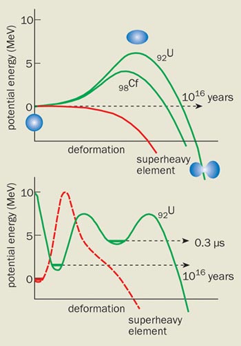
Nuclear fission prompted Niels Bohr and John Wheeler to propose the liquid-drop model, which treats the nucleus as a drop of charged liquid without any structure. As long as the surface tension in the drop is larger than the repulsive Coulomb force due to the protons, a potential barrier prevents it from splitting (figure 1). However, this fission barrier can be overcome if we supply enough energy to the nucleus or if the nucleus “tunnels” through the barrier.
For the uranium-238 nucleus, which has an atomic number of 92, the fission barrier is about 6 MeV high. This leads to a spontaneous-fission half-life of about 1016 years. However, as the atomic number becomes higher, the potential barrier becomes smaller and eventually disappears, causing the heaviest nuclei to decay in about 10-19 s. According to Bohr and Wheeler, the potential barrier disappears completely when the atomic number reaches about 106.
The lifetimes of the first “transuranium” elements – such as plutonium, curium and californium – were very close to the values predicted by the liquid-drop model. In 1962, however, researchers at the Joint Institute for Nuclear Research (JINR) in Dubna discovered that many isotopes of transuranium elements ? which have a very low excitation energy ? undergo spontaneous fission in just 10-10-10-2 s. This is inconsistent with the liquid-drop model predicts. Furthermore, the model could not account for considerable variations in the spontaneous-fission half-lives of these “isomers”.
Researchers soon realized that the probability of spontaneous fission depends on the internal structure of the nucleus. It was well known, for example, that the total nuclear binding energies measured in experiments deviated from the predictions of the liquid-drop model in a regular way. The binding energies were highest for specific numbers of protons, Z = 2, 8, 20, 28, 50, 82, and neutrons, N = 2, 8, 20, 50, 82, 126. These “magic” numbers of protons and neutrons are called closed shells, and are similar to the electron shells of atomic physics.
By the end of the 1960s these observations led to a new microscopic theory of the nucleus, which showed that closed shells of protons and neutrons allow nuclei to be stable beyond the limits defined by the liquid-drop model (i.e. for atomic numbers greater than 106). The shell effect was predicted to be particularly strong for nuclei with magic numbers Z = 108 and N = 162, and even stronger for nuclei with Z = 114 and N = 184 – which is why these regions came to be known as “islands of stability” (figure 2). Indeed, the lifetimes of superheavy nuclei in the N = 184 region are predicted to be up to 30 orders of magnitude longer than they would be in the absence of shells. The challenge presented to experimental nuclear physicists was clear: they needed to create the superheavy nuclei and measure their properties to put the theoretical predictions to the test.
Synthesis reactions
The first transuranium elements were in the main synthesized in successive neutron-capture reactions at the Lawrence Berkeley Laboratory between 1940 and 1953. These experiments – in which nuclei gain extra neutrons during long exposures in a high-neutron-flux reactor – resulted in the discovery of new elements with atomic numbers up to 100 (fermium). However, heavier nuclei could not be explored with this technique because they decayed before they had time to capture the next neutron.
In the effort to produce elements heavier than fermium, researchers turned to heavy-ion reactions, in which two nuclei – one in a heavy-ion beam, the other in a target – are forced to undergo a fusion reaction to create a heavier, compound nucleus. The trouble with this approach, however, is that the collision between the ions leaves the resulting compound nucleus in a highly excited state, which means that it is more likely to undergo fission immediately. Furthermore, the stabilizing effect of nuclear shells decreases rapidly as the excitation energy increases.
Exploring atomic numbers above 106 only became possible after the discovery of so-called cold-fusion reactions at JINR in 1974. In these reactions, heavy ions such as lead or bismuth are bombarded with projectile ions that have a mass number of more than 40. In these reactions, the kinetic energy of the projectile is absorbed, resulting in a compound nucleus that is much less excited.
In the early 1990s Peter Armbruster, Sigurd Hofmann, Gottfried Münzenberg and co-workers at the GSI laboratory in Darmstadt, Germany, used cold-fusion reactions to synthesize elements 107-112. These data were later confirmed by Kosuke Morita and co-workers at the RIKEN laboratory in Tokyo, who also synthesized elements 110 and 111 in cold-fusion reactions. Last year the International Union of Pure and Applied Chemistry (IUPAC) agreed that element 110 should be known as darmstadtium, and that GSI should also be credited with the discovery of element 111. Both the GSI and RIKEN teams now have plans to synthesize element 113 and above.
But even cold fusion has limitations if we want to fully explore the superheavy-element region. This is because massive nuclei tend to resist fusion – an effect that increases with the electric charge of the projectile ion – which means that the probability of forming new elements falls exponentially as
a function of the atomic number of the compound nucleus. Furthermore, the compound nuclei produced in cold-fusion reactions contain a relatively small number of neutrons. In the case of element 112, for example, the final nucleus has 112 protons and 165 neutrons, which is still 19 neutrons away from the predicted closed shell at the magic neutron number N = 184.
One way to produce nuclei with higher neutron numbers is to use the rare isotope calcium-48 – which has 20 protons and 28 neutrons – as the projectile. In these reactions the compound nucleus has an excitation energy of about 30-40 MeV. Although this suppresses the shell effects, they are still strong enough to allow the final superheavy nucleus to be observed. Furthermore, the large mass difference between the two interacting nuclei decreases the Coulomb repulsion between them at the moment they touch, and thus increases the probability of fusion.
Despite these obvious advantages, all attempts to synthesize new elements using calcium-48 ions between 1977 and 1985 failed. However, improved experimental techniques and the availability of intense beams of calcium ions have increased the sensitivity of these experiments by at least three orders of magnitude. This has allowed us, together with colleagues at the Lawrence Livermore National Laboratory in the US, to probe deep into the superheavy-element region.
If the theory is right, elements on the islands of stability should not decay via spontaneous fission. Instead they should undergo alpha decay. As a result, these elements will leave a clear experimental signature: a daughter nucleus that is lighter than its parent by two protons and two neutrons, followed by a granddaughter nucleus that is lighter by four protons and four neutrons, and so on. The decay products of the parent nucleus therefore get further away from the magic numbers Z = 114 and N = 184 until they pass the boundary of the island of stability, beyond which spontaneous fission starts to dominate the decay process. The synthesized heavy nucleus therefore has to be as close as possible to the neutron shell N = 184 to produce a long alpha-decay chain.
Calcium exists naturally in great abundance, but only about 0.19% of it is in the form of neutron-rich calcium-48. Producing this particular isotope is therefore time-consuming and, moreover, it costs about $200,000 per gram. As such, we have had to optimize our accelerator at JINR so that we obtain a high beam intensity for as little calcium-48 as possible.
As a target material we use neutron-enriched isotopes of plutonium (Z = 94), americium (95), curium (96) and californium (98), all of which have long lifetimes. The fusion reaction between these isotopes and calcium-48 allows us to produce elements with atomic numbers between 114 and 118, and neutron numbers between 172 and 177. This is the maximum number of neutrons possible in an element that has been produced artificially. Over a period of five years we have used a total of about 14 g of calcium-48 to create elements 112-116 and also two atoms of element 118 (see Oganessian et al. 2003 in further reading).
In essence, the new heavy elements with Z = 112-118 were all produced at JINR in the same way. To make element 115, for example, we used the reaction 243Am + 48Ca → 291115. The final 115 nucleus contains an odd number of protons and an odd number of neutrons, which considerably reduces the probability that it will decay via spontaneous fission. This means that there is a better chance of observing a long sequence of alpha decays that will give us information about the properties of many nuclei down to Z = 105. An even?even nucleus, on the other hand, is more likely to have short decay chains because it has a higher probability of decaying via spontaneous fission.
Before the crucial fusion reaction can take place the calcium-48 ions need to have enough energy to overcome the Coulomb barrier, which is 236 MeV for this system. However, in order to increase the probability of fusion we used a slightly higher ion energy of 248 MeV, which gave the 291115 nucleus a thermal energy of about 40 MeV.
A compound nucleus with this excitation energy de-excites by emitting three neutrons and gamma-rays to form the isotope 288115, which also has odd numbers of both protons (115) and neutrons (173). As soon as it has formed, the 288115 isotope continues to decay into lighter heavy elements. For instance, after five alpha particles have been emitted we are left with element 105, which is called dubnium.
Once it has been produced in the americium target, the heavy nucleus has a kinetic energy of about 40 MeV and flies through the gas-filled chamber of a magnetic separator. This device directs the nucleus towards the detector, while deflecting the calcium nuclei and other unwanted reaction products. After 1 μs the nucleus is stopped in the front layer of the detector, and about 80 μs later the data-acquisition system gives information on its arrival time, energy and co-ordinates.
About 20-30 s after such an event, our detector registered five further signals, the positions of which were all within 0.5 mm of the heavy nucleus. It then registered nothing until the following day, 28.7 h later, when two signals were obtained from the same position with a total energy of about 200 MeV. In other words, this was the signature of the spontaneous fission of element 105. The long lifetime of the final 105 nucleus, which has N = 163, is due to the closed neutron shell at N = 162.
Decay chains like these were registered three times in total, each of which contained six generations per family: five sequential alpha decays terminated by spontaneous fission. The energy and emission time of the alpha particles
in these three cases were strongly correlated, which means that each decay chain corresponds to the production and decay of the same element. Similar chains were observed when we synthesized the even-Z nuclei of elements 112, 114 and 116, with the lifetimes of the final nuclei in each chain ranging from minutes to hours depending on their proton and neutron numbers. In the absence of nuclear-shell structure, none of these heavy nuclei would exist for longer than about 10-19 s.
The general pattern
We now have data on the properties of 29 new nuclei with atomic numbers between 104 and 118. The decay modes, energies and lifetimes of the heaviest nuclei all agree with the predictions of the microscopic nuclear model, which provides the first experimental evidence for an island of stability in superheavy nuclei.
But we have only reached the shores of this island. We have found a steep rise in the stability of superheavy nuclei with atomic number, but we are still far from the region in which nuclei may live for thousands, maybe even millions, of years. The problem is that we do not yet know how to make the neutron-rich nuclei that will take us towards the magic number N = 184. However, there could be a way round this. If the longest living superheavy nucleus has a half-life of tens of millions years then it should be present in very small quantities on Earth. The only difficulty then is finding it.
One potential candidate for such a long-living element is hassium (Z = 108), which contains about 180 neutrons. In 2001 a team of chemists from Switzerland, Germany and Dubna found that the chemical properties of the short-lived isotope hassium-269 are very similar to those of the dense metallic element osmium (Z = 76), which lies in the same column of the periodic table. The osmium sample might therefore contain a very small quantity of the hassium isotope, which will either undergo spontaneous fission or undergo successive alpha or beta decays until its lighter daughter nuclei undergo fission.
Later this year an experiment led by the present author, in collaboration with researchers in France, will attempt to register these rare spontaneous-fission events in an osmium sample. If our experiment – which is located deep underground in Modane, France, to shield it from cosmic rays – detects just one spontaneous-fission event over a period of one year, we will know that osmium contains an extremely low concentration of element 108. As such we will have found a superheavy element that lies almost on top of the island of stability, which would allow us to test the shell model even further.
In the mean time, we will continue to search for even heavier elements at JINR. We are currently improving the sensitivity of our experiment and increasing the intensity of the beam. Ultimately, however, we will need to use a heavier projectile than calcium-48 if we want to stretch the boundaries of the periodic table even further.
Conventional ultrasound techniques involve sending a series of sound pulses into the body and monitoring the reflections of these pulses from tissue boundaries. By measuring both the time taken for each pulse to return to the source and the amplitude of each pulse, ultrasound machines can build up an image of these boundaries. However, while this approach is ideal for generating images of the outlines of organs, it provides little information about the types of tissue within these organs. For example, a doctor may be able to use an ultrasound image to identify a tumour by virtue of its shape, but may be unable to tell whether it is benign or not.
This limitation stems from the way that sound travels through different materials. Solid materials can be regarded as a matrix of point masses interconnected by springs. Sound waves propagate through such materials by periodically compressing and rarefying the medium. The speed of sound through a particular material therefore depends on the material’s spring constant, or elastic modulus. Although the value of the modulus varies significantly between bone and skin, for example, it does not vary much between different types of soft tissue. This means that contrast between such materials in an ultrasound image is poor.
The advantage of the new approach is that the elastic modulus associated with shear waves varies greatly between different types of tissue.
In the July issue of Physics World Peter Kaczkowski of the Applied Physics Lab at the University of Washington in Seattle describes this work in more detail.