At room temperature, the extraordinary magnetoresistance of such non-magnetic materials is much larger than that of other magnetic materials, including those that exhibit giant or colossal magnetoresistance. Now Joseph Heremans and co-workers at Delphi Research Laboratories in Michigan, US, have shown that there can also be a significant geometric contribution to the so-called magnetothermopower of indium antimonide (J P Heremans et al. 2001 Phys. Rev. Lett.86 2098).
In the June issue of Physics World, Stuart A Solin of the NEC Research Institute, US, explains the new effect.
Enormous advances in solar and stellar physics have been made in recent years as a result of helioseismology – the study of vibrations on the surface of the Sun. However, the Sun is only one star among many. While we believe it is a typical star, we do not know for certain. What we need are observations of the oscillations in other solar-like objects. Sadly such studies are difficult because all other stars are far away and the oscillations are very small. Now Tim Bedding of the University of Sydney and co-workers in Australia, the US, Denmark and Switzerland have announced the detection of solar-like oscillations on Beta Hydri – a star much like our Sun, except that it is older and more evolved (T Bedding et al. 2001 Astrophys. J.549 L105). Although other groups had previously claimed to have detected oscillations on other Sun-like stars, most solar and stellar seismologists felt that these results were not robust.
In the June issue of Physics World, Yvonne Elsworth of the University of Birmingham, UK, discusses why the results of Bedding and co-workers, in contrast, look very promising.
Last year our group at the California Institute of Technology teamed up with Loren Pfeiffer and Ken West of Bell Labs to study how electrons tunnel between two parallel 2-D electron gases. These electrons reside in a semiconductor heterostructure consisting of two thin layers of gallium arsenide separated by a barrier layer of aluminium gallium arsenide. Surprisingly, we observed a huge enhancement in the tunnelling current when just the right magnetic field was applied perpendicular to the 2-D planes in which the electrons were confined (I B Spielman et al. 2000 Phys. Rev. Lett.84 5808).
In the June issue of Physics World, James P Eisenstein of the California Institute of Technology, USA, describes the experiment and explains where it may lead.
The real show-stopper for science is a shortage of school teachers in general, and a chronic shortage of science teachers in particular, that threatens the economic prosperity of the country in a knowledge-based world. The new government has it in its power to increase salaries for teachers and, at the same time, reduce the administrative burdens that have had such a demotivating effect on the profession.
Attempts to increase the number of young people going to university are also being hampered by the fact that most students now graduate with debts that run into thousands of pounds. At the last election in 1997 all the major parties were vague about their higher-education policies because the Dearing committee – which was conducting the biggest review of higher education in 30 years – had not then produced its final report. However, the Labour government effectively ignored most of Dearing’s recommendations on student finance to produce a botch job – replacing grants with loans and introducing limited fees – that has pleased no one. Some form of graduate tax is surely the way forward, but it is difficult to imagine any of the parties having the vision or the guts to float such an idea.
What about academics? Their salaries are not competitive in international terms, which means that UK universities can no longer attract the brightest talents, although moves have recently been made to address this problem. However, Labour has allowed too many onerous reviews of the universities, such as the Quality Assurance Agency’s reviews of teaching quality and the “transparency” review of money spent on teaching and research.
However, the Labour government must be given credit for its willingness to invest new money in the science base. The fact that British astronomers are currently negotiating to join the European Southern Observatory is a refreshing change from the early 1990s when the Conservative government of the time seemed intent on pulling out of as many European ventures as possible. It is essential that this enlightened and far-sighted approach continues, and that the next government also does what it can to encourage British industry to invest in R&D at the same levels as its competitors.
Thomas Young lives on
Some 200 years ago a young polymath and qualified medical doctor called Thomas Young turned his attention to light. Young had already made several medical breakthroughs – he discovered the cause of astigmatism, for instance, but his medical career was unsuccessful because he lacked a suave bedside manner – when he became the first physicist to demonstrate that light is a wave. Not surprisingly, Young’s famous double-slit interference experiment was initially met with hostility because the wave theory of light ran counter to Newton’s corpuscular theory. Now, of course, we know that both were right.
Young went on to make many other discoveries in optics, elasticity and other areas of physics – not to mention helping to decipher the Rosetta stone – and, as this month’s feature on quantum carpets illustrates, the subject of interference continues to fascinate physicists 200 years later.
Cosmologists aren’t shy of making bold claims about their subject. Paul Steinhardt of Princeton University, for example, believes that we are living through a “revolution” in our understanding of the universe as profound as that brought about by Copernicus. His convictions have been bolstered by results announced at the end of April from three independent experiments measuring the so-called cosmic microwave background (CMB). The results show that sound waves propagated through the early universe in a series of harmonics, as predicted by the established theory of the universe’s origins – inflationary big-bang theory.
“The latest CMB measurements are a stunning vindication of our understanding of the universe,” says cosmologist Michael Turner of the University of Chicago. “We are now making measurements of a high enough precision that we can test predictions of bold ideas. These measurements show that inflation is passing with flying colours.”
Inflation was first proposed by Alan Guth of the Massachusetts Institute of Technology in 1981. According to this theory, the very early universe expanded exponentially for about 10-32 seconds, before settling down to a slower rate of expansion. In the process, quantum fluctuations were stretched out into the density variations that eventually led to all the structure in the universe, from galaxies to humans. The three experiments – called Boomerang, DASI and Maxima (an international and two American collaborations, respectively) – detected these density variations in the CMB, the microwave remnant of the radiation produced about 300 000 years after the big bang (see box).
Turner admits that it is “too early to crown the inflationary model”, but is confident that it will see off the competition. The new data rule out several alternative models of the universe’s evolution known as topological defect models, since these theories predict that structure was seeded more than 300 000 years after the big bang.
However, not everyone is so sure about inflation. John Peacock of Edinburgh University, for example, points out that the data do not rule out other theories that propose a quantum origin to structure. “The peaks [in the CMB] were predicted ten years ahead of inflation. To say that they are strong evidence for inflation itself is wishful thinking,” says Peacock. “The CMB is verification that we understand how structure in the universe has developed since the universe was 103 times smaller than at present – but inflation is presumed to have happened when the universe was 1028 times smaller than today, so there is still a long way to go.”
Mike Disney, a cosmologist at Cardiff University, is also sceptical of inflation theory, which he likens to our understanding of the solar system. “The celestial motion of the planets can be traced with wonderful precision but this doesn’t mean we know how the solar system formed,” he says. “I am very impressed with the Boomerang data but this doesn’t mean we know everything about the evolution of the universe.”
A snapshot of the primordial universe
Microwave snapshot of the CMB.
The early universe consisted of a hot, dense plasma containing photons, electrons, protons and a small amount of helium and other light elements. The photons repeatedly scattered off the electrons and were therefore restricted to the plasma. But when the universe was about 300,000 years old it had expanded and cooled to below 3000 K – low enough to allow atomic hydrogen to form. In the absence of free electrons, the photons were able to travel freely through the expanding universe. The background radiation that we detect today is therefore a record of the universe as it was just 300,000 years after the big bang, but it has been stretched, or “red-shifted”, to its current microwave wavelength due to the universe’s expansion.
The density variations caused by inflation manifest themselves as hot and cold patches in the background radiation. This is because the differences in density set up compressions and expansions in the primordial plasma, which propagated as sound waves, causing the gas to heat up when compressed and cool when expanded. The Cosmic Background Explorer satellite first detected these patches in 1992 as temperature variations of just one part in 105 in the microwave radiation, which it showed had a perfect black-body spectrum with a temperature of 2.73 K.
An analysis of the data from the Boomerang and Maxima experiments that was published last year confirmed the presence of the largest patches, which extend about a degree across the sky. But there was no firm evidence for higher “harmonics” – the patches that are predicted to occur at smaller angular scales. These have been seen in the latest data (see image above). They are also represented as peaks in a graph of the amplitude of temperature fluctuations against angular scale, i.e. how many ripples there are of a given size. The first, and largest, peak lies at about a degree, the second at about 0.4 degrees and the third at about 0.25 degrees.
Putting inflation to the test
Altogether over 30 experiments to measure the CMB have been completed, are in operation or are planned. Until now these have been small-scale affairs – some of which have been ground-based, such as DASI, located at the South Pole, and most of the rest – such as Boomerang and Maxima – have been suspended from balloons. But that will change this month with the launch of NASA’s $145m satellite called the Microwave Anisotropy Probe (MAP). This will be some 100 times more accurate than previous experiments and will record images of the CMB across the whole sky. Boomerang, in comparison, covered only about 3% of the sky.
“The idea is to get as much information out of the CMB as possible,” says Turner. “Unlike the balloon experiments, MAP will not suffer from atmospheric interference and will have no calibration problems.” Since it will study the whole sky, MAP will be able to calibrate its voltage measurements using a pair of well known hot and cold spots in the heavens.
Chuck Bennett, the principal investigator on the MAP mission, believes the NASA satellite will significantly improve our knowledge of the universe. “MAP is in a different category to current experiments. It will make a full sky map with unprecedented precision and accuracy to determine the history, content, shape and fate of our universe.”
But the excitement does not stop there. In 2007 the European Space Agency will launch the Planck satellite. It will measure temperature fluctuations some three times smaller than the smallest to be studied by MAP, and will be the first serious attempt to measure the polarization of the CMB.
Measuring the CMB’s polarization will be a major test of inflationary theory. The gravity waves that would have been created by the huge expansion of matter in the inflationary universe lead to a distinctive pattern of polarization. But rival theories would not necessarily involve the formation of gravity waves. The “ekpyrotic” theory, for example, which has recently been put forward by Steinhardt and colleagues, proposes that our universe was kicked into life by an offshoot of a hidden parallel universe subject to random quantum fluctuations. This does not involve a rapid expansion of the early universe and therefore disturbances in the gravitational field have properties that differ from those predicted by inflation.
Planck will also provide another major test of inflation by measuring the so-called scale invariance of the fluctuations in the CMB to better than 1%. (MAP could measure gravity waves or scale invariances in principle, but existing data suggest it may not be accurate enough.) Scale invariance is calculated by measuring the relative amplitudes of the fluctuations in the CMB. If the universe is scale invariant then the size of density perturbations, which are related to the temperature fluctuations, is independent of the angular scale. Inflation predicts that the perturbations will have a small, but measurable, deviation from exact scale invariance.
Precision cosmology
Measuring something to within 1% may not sound like anything to be proud of. In particle physics, for example, researchers need to reduce errors to three parts in 10 million in order to claim the discovery of a new particle. But 1% is a big deal in cosmology, a subject more used to measurements that are in error by several hundred per cent. In fact, the improvement in the measurement of scale invariance that Planck will obtain should be enough to test the validity of inflation.
What gets cosmologists excited about the CMB, however, is not just the accuracy of the measurements in isolation but that the data fit into an overall framework supported by a range of cosmological observations. “We are now in a wonderful position in cosmology because results from different kinds of measurement are fitting together in a coherent whole, such as those from the CMB and supernovae,” says Steinhardt.
By measuring the relative amplitudes of the temperature fluctuations at the largest angles, cosmologists have calculated that ordinary, or “baryonic”, matter accounts for about 5% of the universe’s total mass and energy. This figure agrees with an estimate of the amount of ordinary matter in the universe based on calculating the quantity of deuterium produced in the big bang.
“The agreement between measures of the amount of ordinary matter is simply stunning,” says Turner, “even though the underlying physics is completely different. The big-bang framework and Einstein’s general relativity have passed a major new test.”
The new CMB data also support the idea that the geometry of the universe is flat, which means light travels in straight lines. The universe consequently has a “critical” energy density since any deviation from this density would mean light following a curved trajectory. This is important because it is consistent with observations of the more recent universe.
In particular, observations of galaxies, such as those contained within the “two-degree field” survey being carried out by British and Australian astrophysicists, show that the total amount of matter – baryonic plus exotic dark matter (matter not made up of electrons, protons and neutrons) – is only about one-third of the critical energy density. It is thought that the remaining two-thirds of the energy density is made up of a mysterious substance called “dark energy”, which would act like negative gravity. If the total energy density consisted entirely of matter, the consequent gravitational potential would cancel the kinetic energy of the universe, and the universe’s expansion would eventually grind to a halt. But the dark energy means instead that the universe’s expansion ought to accelerate.
Such an acceleration has indeed been observed in distant supernovae, which ties the loose strands together and makes cosmologists happy. “The dark-energy revolution is as important as the Copernican revolution,” says Steinhardt. “Copernicus challenged our perception of our place in space. Dark energy challenges our place in time.”
This view is not shared by everyone. Joseph Silk, an astrophysicist at Oxford University, stresses that dark energy remains a working hypothesis. “I am not going to work on this,” he says. “I hope dark energy will go away. It has come and gone over the years. It all remains to be confirmed.” He does admit, however, that “the evidence is piling up, and looks more and more convincing”.
Cosmologists are sceptical about dark energy, not least because no-one knows what it actually is. One possibility is the “cosmological constant” that Einstein introduced as a fudge factor in general relativity to explain what was presumed to be a static universe (he described this as his “greatest blunder” following Hubble’s observations of the expanding universe). Another possibility is something known as “quintessence”. Both alternatives would consist of vacuum energy, but the latter would evolve over time. A comparison of the vacuum density today with that imprinted in the CMB should therefore tell researchers the correct model, a calculation that may be possible with measurements from MAP and Planck.
Disney points out that new observations could not only bolster current theories, but may completely overhaul current thinking. “Originally scientists thought we lived in a static universe. But experimental evidence proved otherwise,” he says. “The universe is a more complicated place than theorists like to think. In 20 years time’ we will still be wondering about the big questions.”
Turner agrees that people will still be searching for cosmic answers in 20 years’ time, but believes that inflation, dark energy and cold dark matter will hold firm. “I’m more than cautiously optimistic that inflation theory will still be around come the end of the Planck mission,” he says. “It is true that the only surprise in this golden age of cosmology would be no more surprises. But I don’t think there will be any surprises to topple the whole framework.”
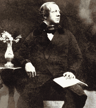
Henry Fox Talbot: 1800–1877. (Picture courtesy of The National Trust and the Fox Talbot Museum, and kindly supplied by Michael Gray)
In 1836 Henry Fox Talbot, an inventor of photography, published the results of some experiments in optics that he had previously demonstrated at a British Association meeting in Bristol. “It was very curious to observe that though the grating was greatly out of the focus of the lens…the appearance of the bands was perfectly distinct and well defined…the experiments are communicated in the hope that they may prove interesting to the cultivators of optical science.”
Talbot made his remarkable observation as he inspected a coarsely ruled diffraction grating, illuminated with white light, through a magnifying lens. With the lens held close to the grating, the rulings appeared in sharp focus, as expected. Moving the lens away, so that the grating was no longer in focus, the images should have become blurred but instead remained sharp. Moreover, the images consisted of alternating bands, the complementary colours (e.g. red and green) of which depended on the distance of the lens from the grating.
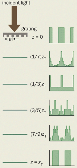
As the lens receded further, the sequence of colours repeated several times over a distance of the order of metres. With monochromatic light, the rulings of the grating first appeared blurred, as expected, but then mysteriously reappeared in sharp focus at multiples of a particular distance, zT (figure 1).
Forgotten for decades
1 Talbot and his diffraction effect The Talbot effect from a Ronchi grating – a grating that has equally spaced transparent and opaque slits. The intensity pattern at the grating (z=0) is reconstructed at the Talbot distance z=z1 but is shifted by half a period. The images that can be viewed with the aid of a lens (not shown) occur at intermediate distances given by rational fractions p/q of zT. These “fractional Talbot images” consist of q overlapping copies of the grating; several values of p/q are illustrated here. Neighbouring images are shifted by a/q, and coherently superposed with phases given by the Gauss sums of number theory (see box).
This “Talbot effect” – the repeated self-imaging of a diffraction grating – was forgotten for nearly half a century until it was rediscovered by Lord Rayleigh in 1881. Rayleigh showed that the so-called Talbot distance, zT, is given by a2/L, where a is the slit spacing of the grating and L is the wavelength of the light. For red light with a wavelength of 632.8 nm and a grating with 50 slits per inch (a = 0.508 mm) the Talbot distance is 407.8 mm. Rayleigh pointed out that the Talbot effect could be employed practically to reproduce diffraction gratings of different sizes by exposing photographic film to a Talbot-reconstructed image of an original grating. Then the Talbot effect was forgotten again.
Recent investigations have revealed that the Talbot effect is far more than a mere optical curiosity. First, the effect is one of a class of phenomena involving the extreme coherent interference of waves. Second, these phenomena have deep and unexpected roots in classical number theory. And third, they illustrate something we are starting to appreciate more and more, namely the rich and intricate structure of limits in physics.
And who was Talbot? He is best known for his invention of photography, independently of French physicist Louis-Jacques-Mandé Daguerre, rather than the physics of diffraction gratings. And it is Talbot’s process, involving a negative from which many positive copies can be made, that we use in all non-digital photography today. But Talbot did much more: as an English landowner and parliamentarian, he ran the family estate at Lacock; he was one of the inventors of the polarizing microscope that has been indispensable to mineralogists; he proved theorems about elliptic integrals; and he contributed to the transcription of Syrian and Chaldean inscriptions.
Quantum revivals
2 Quantum revivals Quantum carpets, i.e. plots of probability density, for the propagation of a Gaussian wavepacket in a 1-D box with length x = 1. The horizontal axes are the coordinate x and the vertical axes are t/Tr where t is time and Tr is the revival time. (a) One period of the quantum carpet; (b) magnification of (a) for short times, showing the initial packet bouncing in the box as it spreads: (c) magnification near Tr/2, showing fractional revival of two copies of the initial packet. The intensity increases with brightness and saturation, and is colour-coded with hue (maxima represented by red). These carpets are calculated using the equation in the box below, for w = 1/10, k = 20 (thus giving a classical period Tc = Tr/20).
There is a phenomenon in quantum physics that is closely related to the Talbot effect. A quantum wave packet – representing an electron in an atom, for example – can be constructed from a superposition of highly excited stationary states so that it is localized near a point on the electron’s classical orbit. If the packet is released, it starts to propagate around the orbit. This propagation is guaranteed by the correspondence principle: for highly excited states, quantum and classical physics must agree. The packet then spreads along the orbit, and eventually fills it. (It also spreads transversely – that is away from the orbit – but that is not important in this context.)
Over very long periods of time, however, something extraordinary happens: the wave packet contracts and after a time, Tr, returns from the dead and reconstructs its initial form. This is a quantum revival. As time goes on, the revivals repeat. In a wide class of circumstances, the reconstructions are almost perfect.
3 Talbot carpets and mountains (a) A carpet of light from a Ronchi grating. A density plot of Talbot intensity in a single period transversely (across the grating) and longitudinally (along the direction of the incident light). The colour coding is the same as in figure 2. Note that the grating and associated interference patterns have reappeared at z = zT but shifted by a half-period. (b) The mountains of Talbot. A visualization of the intensity in (a) as a surface.
In the Talbot effect, the pattern of intensity is doubly periodic, both across the grating and as a function of distance from the grating. Similarly, for quantum revivals the probability density is both periodic around the nucleus and as a function of the time evolution of the wave packet. These periodicities are the result of coherent interference. Rayleigh understood this for gratings (where the interference is between the wavelets from the different slits), and there is a similar result for revivals. For a packet consisting of hydrogen-like states close to the nth energy level, En, the revival time is of the order of nTc, where Tc = hn3/2E1 is the orbital period of a classical electron and h is Planck’s constant. Because of these periodicities, the intensities can be depicted as repeating patterns in the plane that resemble exotic carpets or alien landscapes (figures 2 and 3).
Now comes the number theory. In addition to the reconstructed Talbot images at z = zT and quantum revivals at t = Tr, there are more complicated reconstructions at fractional multiples of the Talbot distance and the revival time. The Talbot image at distance (p/q)zT is a superposition of q copies of the initial grating separated by a/q (figure 1). Thus if p/q = 3/5, there are five superposed images. This is the fractional Talbot effect. And the quantum wave at time (p/q)Tr is a superposition of q copies of the initial wave packet, separated by an angular distance 2 pi/q. These are the fractional revivals.
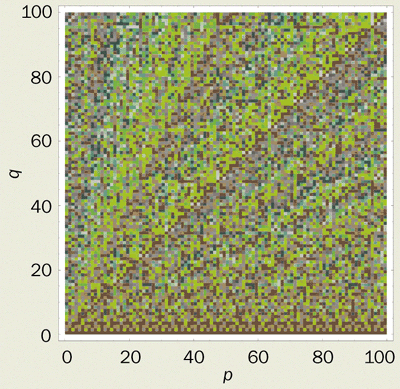
4 Gauss sums Phases of Gauss sums for the n – 2 Talbot image (see box), colour-coded by hue. Red represents a phase of zero, while light blue represents phases of ±π.
At the heart of the rather complicated mathematical explanation of this remarkable phenomenon is the simple identity (-1)n2 = (-1)n, where n is an integer that labels the contributing wavelets. The application of this identity greatly simplifies the sums over the contributing wavelets. Each image in a reconstruction has the same amplitude, 1/q1/2, and its phase is given by beautiful sums discovered by Gauss at the end of the 18th century (see box). In words, the phase of the nth image is the direction of the resultant vector when q unit vectors are added in the complex plane. The angle between the first pair of vectors is 2 pi n/q (plus a constant that does not depend on n) and decreases by 2 pi p/q for each successive pair. The rich patterns of the carpets originate in the complicated patterns of the phases of the Gauss sums (figure 4).
On closer inspection, diagonal “canals” can be seen criss-crossing the carpets. In Talbot carpets, the canals are minima of intensity that are correlated between neighbouring image planes. In quantum carpets, they are space-time structures corresponding to features of the wave that move at fixed velocities (unrelated to the speed of the classical packet). The canals can be understood in several equivalent ways: in terms of destructive interference between positive- and negative-order diffracted beams (that is Fourier components of the patterns); by the transverse structures that remain after averaging along the anticipated directions of the canals; and by arguments involving position and momentum simultaneously (through the evolution of Wigner functions in phase space).
Fractal carpets
Both Talbot and quantum carpets can have intricate fine structure. Consider the case where the transparency of the grating is discontinuous, as it is in the Ronchi grating where the rulings consist of sharp opaque and transparent bars. Alternatively imagine that the quantum wave is discontinuous, as for a particle in a box where the initial wave amplitude plummets to zero at the walls, even though it varies smoothly inside the box.
In Talbot terminology the reconstructed images in the plane z = (p/q)zT consist of q superposed copies of the grating, complete with discontinuities. Although there is an infinite number of images at fractional distances, they still represent an infinitesimal subset of all possible images.
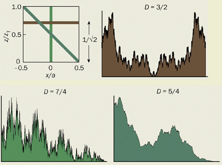
5 Fractal Talbot intensities Talbot fractals from a Ronchi grating. The graphs of intensity have fractional dimensions D. Transverse fractals have D = 3/2 (in planes of constant z that are separated from the grating by distances that are irrational fractions of zT). Longitudinal fractals have D = 7/4 (in sections where x is constant), while diagonal fractals have D = 5/4.
What happens in planes that are irrational fractions of the Talbot distance, for example zT/21/2? The light intensity is then a fractal function of distance x across the image. To be precise, this means that the graph of intensity as a function of x, regarded as a curve in the plane, is continuous but not differentiable. In other words, although the intensity has a definite value at every point, the curve has no definite slope and so is infinitely jagged. Such curves are described as having a “fractal dimension”, D, between one (corresponding to a smooth curve) and two (corresponding to a curve so irregular that it occupies a finite area). Carpets generated by Ronchi gratings, for example, have a fractal dimension of 3/2 (figure 5).
Carpets are functions of the longitudinal coordinate z (along the propagation direction) as well as the transverse coordinate x, so the wave intensities can be plotted as surfaces on the x–z plane (see figure 3b, for example).
What is the fractal dimension of these Talbot or quantum landscapes? As these landscapes are surfaces, they have a dimension that takes a value between two and three. For a surface where all directions are equivalent, the dimension of the surface is one greater than the dimension, D, of a curve that cuts through it. For a Talbot landscape, where the fractal image curves have D = 3/2, we might expect the dimension to be 1 + 3/2 = 5/2.
But Talbot landscapes are not isotropic. For fixed x, the intensity also varies as a function of distance z from the grating, with a fractal dimension of 7/4 (figure 5). Therefore the longitudinal fractals are more irregular than the transverse ones. Finally, the intensity is more regular along the diagonal canals because of the cancellation of large Fourier components and has fractal dimension of 5/4 (figure 5). The landscape is dominated by the largest of these fractal dimensions, and so is a surface with dimension 1 + 7/4 = 11/4.
This fractal structure also applies to the evolving wave from a particle in a box with uniform initial wave amplitude. There are space fractals (varying x with constant t), where the graph of the probability density has D = 3/2; time fractals (varying t with constant x), where the graph of the probability density has D = 7/4; and space-time fractals (along the diagonal canals), where D = 5/4. Some of these results about fractals can be generalized to waves evolving in enclosures of any dimensions, even with shapes that do not give rise to revivals, provided the initial state is discontinuous, even if only at the boundary.
Asymptotic physics
There is, however, a sense in which the carpets – at least as we have described them – are fictions. Like all calculations in physics, they rely on approximations that are valid only in certain limiting circumstances. For a start, the perfect Talbot reconstructions, and the ideal fractals in the case of gratings with sharp-edged slits, depend on the illuminating wave being perfectly plane and infinite in extent.
Obviously this is not true in practice, and corrections can be calculated. For N illuminated slits, the finest details of the reconstructed images and of the fractals are blurred transversely by Delta x ~ a/N and longitudinally (i.e. in the depth of focus of Talbot images) by Delta z ~ zT/N2.
More fundamental is the fact that the finite wavelength of the light, L, must limit the fine detail in the optical field, so that even with infinitely many slits the images would still be blurred.
Perfect reconstruction is an artefact of the paraxial approximation, in which the deflections theta of all relevant diffracted beams are assumed to be small, so that cos theta ~ 1 – theta2/2. Deviations from this approximation get smaller as the ratio L/a decreases, that is in the short-wave limit, or for coarse gratings. The blurring in both the transverse and longitudinal directions is of the order of (aL)1/2. However, the blurring in z is much smaller relative to the periodicity in the pattern because the detail is stretched over the Talbot distance, which greatly exceeds the slit spacing.
These blurrings should not be confused with the more familiar Fresnel diffraction of light from a single edge of a slit, which would be of order a in the transverse direction at z = zT. An alternative way to state the Talbot effect is that the Fresnel blurring from the edges of all the slits is cancelled by the coherent interference of the waves.
In the quantum case, the perfection of the revivals is degraded by an effect that seems different but is mathematically very similar. Analogous to the paraxial approximation is the assumption that the energy can be approximated by terms that are both linear and quadratic functions of the quantum number n, over the range of energies included in the initial state. (If the variation were merely linear, then the wave packet would not spread at all.)
In the case of a non-relativistic particle in a box, the revivals are perfect because the variation in energy is quadratic. However, quadratic variation only approximately describes an electron in an atom: the approximation is semi-classical, that is it gets better as the quantum number, n, corresponding to the central energies in the packet increases. Non-quadratic corrections to the spectrum degrade the revivals, in ways that are now well understood.
Paradoxical limits
Quantum and optical carpets provide a dramatic illustration of how limits in physics that seem familiar can in fact be complicated and subtle. It is no exaggeration to say that perfect Talbot images, and infinite detail in the Talbot fractals, are emergent phenomena: they emerge in the paraxial limit as L/a approaches zero.
At first this seems paradoxical, because the short-wave approximation is usually regarded as one in which interference can be neglected, whereas the Talbot effect depends entirely on interference. The paradox is dissolved by noting that the Talbot distance increases as the wavelength approaches zero, so here we are dealing with the combined limit of short wavelength and long propagation distance: in the short-wavelength limit, the Talbot reconstructed images recede to infinity.
6 Talbot reconstructed caustics A phase grating that produces a sinusoidal wavefront. The geometrical-optics rays and caustics are shown in (a) while the resuIting TaIbot carpets, i.e. density plots, are shown in (b)-(e). (b) One period of the Talbot carpet; (c) half-period of the Talbot carpet; (d) anisotropic magnification shows a geometrical caustic near the grating; (e) anisotropic magnification shows one of the Talbot-reconstructed caustics near z/zT = 0.5. The colour coding is the same as in figure 2. The carpets are calculated using the equation in the box for λ/H = 1/(400π2).
In a similar way, perfect quantum revivals emerge from the semi-classical limit of highly excited states. Again it might seem paradoxical that an interference effect persists in a semi-classical limit (and indeed emerges perfectly in that limit). The dissolution of the paradox is analogous to that in the Talbot case: the semi-classical limit here is combined with the long time limit (recall that Tr ~ nTc), so the revivals occur in the infinite future.
Even within the paraxial approximation, a clash of limits can generate very rich phenomena. Consider a transparent phase grating, that is a diffraction grating that transmits light with uniform amplitude but introduces a sinusoidal phase variation with period a.
In the geometrical-optics approximation, light rays passing through the grating are deflected so that they are normal to the sinusoidal wavefront that is generated immediately beyond the grating. These rays generate the pattern shown in figure 6a, which is dominated by caustics, i.e. curves onto which the light is focused and in which the intensity is concentrated.
Pairs of caustics join at cusps located near the centres of curvature of the wavefronts. The resulting pattern of rays is not periodic in z, and is thus discordant with the notion that the pattern of waves must repeat with period zT for the Talbot effect to occur. Again the paradox is dissolved by the observation that the Talbot distance is of the order of 1/L, and so recedes to infinity in the geometrical-optics limit where L tends to zero.
However, when L/a is small but non-zero, both the caustics and the Talbot repetitions must coexist. This means that the geometrical caustics, including the cusps for distances much less than the Talbot distance, must be regenerated at both integer multiples and fractional multiples of zT. Figures 6b and c show the Talbot carpet for this sinusoidal grating, with apparently no trace of the geometrical-optics caustics and their cusps.
However, appropriate magnification shows that the original and regenerated caustics (and associated diffraction fringes associated with a single sinusoid) are indeed hidden in the detail of the carpet (figures 6d and e). It is worth emphasizing what a remarkable phenomenon this regeneration is: geometrical-optics caustics have been constructed entirely by interference, in regions where there are no focusing rays. They are the ghosts of caustics. There is a curious analogy between these “caustics without rays” and Moiré patterns, which are “fringes without waves”.
Experiments and outlook
These predictions – Gauss sums, waves reconstructing themselves, fractal carpets and canals – are not just arcana from the imaginations of theorists. Many of the results have been confirmed by experiments.
Fractal aspects of Talbot interference were seen in optical experiments by one of us (MB) and Susanne Klein of Bristol University in 1996. Fractional Talbot images were seen in matter waves (a beam of helium atoms) diffracted by a microfabricated grating, in experiments carried out at the University of Konstanz in 1997 by Stephan Nowak, Christian Kurtsiefer, Christian David and Tilman Pfau.
And fractional quantum revivals have been seen in electrons in potassium atoms, which were knocked into appropriate initial states by laser pulses using a “pump-probe” technique. These experiments were performed by John Yeazell and Carlos Stroud at the University of Rochester in 1991. Analogous observations of the vibrational quantum states of bromine molecules were carried out in 1996 by Max Vrakking, David Villeneuve and Albert Stolow at the University of Ottawa in Canada.
There are also the beginnings of applications for technology. Following Rayleigh’s pioneering example, the fine detail in Talbot wavefunctions is being employed in lithography. And the number-theory properties of the phases have been proposed as the basis of a means to carry out arithmetic computations based on interference.
However, the predicted Talbot reconstruction of caustics for smooth phase gratings has yet to be observed. An appropriate grating for such experiments could be a sheet of glass with an undulating surface, or a wave on water. And as the manipulation of electronic and molecular wave packets with ultra-short laser pulses gets more sophisticated, we envisage more detailed experimental exploration of the fine structure of the carpets, such as the diagonal canals.
The optical field behind a coherently illuminated diffraction grating, and the quantum particle in a box with uniform initial state, are two of the most venerable and widely studied systems in physics. It was quite unexpected to discover such richness hidden in them, and also to see it displayed by such a wide range of physical systems. Further exploration of these intricate manifestations of the coherent addition of waves is a fitting way to celebrate the bicentenary of Thomas Young’s great discovery of the interference of waves of light.
Formulas used to calculate quantum revivals and carpets
Quantum revivals (figure 2): for an initial packet with width w starting from x = 1/2 and with momentum k, the wave is (up to a constant factor)
Talbot carpet (figures 1b, 3 and 5): the wave from a Ronchi grating is
Talbot carpet (figure 6): the wave from a phase grating producing a sinusoidal wavefront with amplitude H is
where the Jn are Bessel functions.
Gauss sums (figure 4): For the nth superposed Talbot image at distance z = (p/q)zT, the phase is chi(n;p,q), defined by
where e(p) = 0 if p is even and e(p) = 1 if p is odd.
Phase transitions in nuclei are difficult to understand because of the many degrees of freedom involved, so theorists have had to rely on complex numerical calculations that contain many free parameters. To understand these nuclei fully, however, physicists need a mathematical model that can describe their different properties without a large number of guiding assumptions. Iachello has now developed such a model – which he calls X(5) symmetry – for spherical nuclei that transform into a rugby-ball shape during a phase transition. By solving the Schrodinger equation at the critical point – the point where both states co-exist – he can predict the properties of phase-transition nuclei by simply plugging in their quantum numbers. The theory could also be applied to metallic clusters, molecules and polymers.
By chance, recent experiments at Yale, Cologne University in Germany and the Institute Laue-Langevin in Grenoble, France, hinted that samarium-152 nuclei undergo exactly the right type of phase transition. With 62 protons and 90 neutrons, these stable nuclei were thought to lie close to the critical point. Casten and Zamfir have now taken a closer look at the energy levels of excited samarium-152 nuclei, and the strengths of the transitions between them. In general, they found an excellent agreement between the measurements and X(5) symmetry. They also found that neodynium-150, like samarium-152, co-exists as spherical and rugby-ball nuclei.
“This is one of the most interesting things I have ever done,” Casten told PhysicsWeb. X(5) symmetry gives experimentalists a new benchmark against which to test nuclei. With the production of ever more exotic nuclei at radioactive beam facilities, Casten believes that the latest work has a good chance of “starting a new direction in nuclear physics”.
The transition temperature of magnesium diboride is 38 K – almost double that of any other metallic superconductor. Wires and tapes made from the new compound could therefore potentially be cooled with electrical refrigerators, which are relatively cheap, rather than cumbersome liquid-helium cooling systems. However, in its pure bulk state magnesium diboride cannot superconduct when carrying significant currents or when exposed to large magnetic fields. A magnetic field creates vortices within the material, the cores of which behave as simple conductors. When the magnetic field is high enough the vortices spread throughout the whole of the material and all superconductivity is lost. In addition, current flow moves the vortices, producing friction within the atomic lattice and so creating resistance.
However, such resistance can be overcome by defects in the material, which “pin” vortices and prevent them from moving. Now three teams of researchers have exploited this pinning effect to increase both the maximum or critical current, Jc, that the material can withstand in its superconducting state, and the irreversibility field, H*, above which resistance free currents are no longer possible.
By studying thin films of oxygen-doped magnesium diboride, Chang-Beom Eom of the University of Wisconsin in the US and colleagues obtained values of the irreversibility field that were double those observed in the bulk material (C Eom et al. 2001 Nature411 558). They also significantly increased the critical current density to 100000 amps per square centimetre at 4.2 K and 10 Tesla. It is thought that the interface between the thin film and its substrate creates pinning defects in this material.
Meanwhile Yury Bugoslavsky of Imperial College in London and the General Physics Institute in Moscow, and colleagues, produced vortex pinning by irradiating samples of magnesium diboride with protons (Y Bugoslavsky et al. 2001 Nature411 561). This group was also able to double the value of the irreversibility field and observed a much slower reduction in the critical current with applied field at 20 K.
Finally, a group at Lucent Technologies led by Sungho Jin has reported a critical current of 30000 amps per square centimetre at 25 K and 1 Tesla by cladding a sample of magnesium diboride in iron (S Jin et al. 2001 Nature411 563). The vortex pinning in this case may have been due to the crushing and rolling used to draw the superconducting wire.
The second is currently defined as the time taken to complete 9192 631 770 oscillations between two energy levels in a caesium atom. The current generation of caesium clocks boast an accuracy of one part in 1015 – equivalent to an error of less than one second in 30 million years. However, this accuracy could be improved by several orders of magnitude if optical transitions were used to measure time rather than microwave transitions in caesium. The main problem when building an optical clock is to relate these optical frequencies to the much lower microwave frequencies that are used to define the second – a task that once required an extremely complex “frequency chain”.
Last year Udem, then at the Max Planck Institute for Quantum Optics in Garching, near Munich, and colleagues at Garching and Bath University in the UK, developed a “frequency comb” that made this task much easier. To make the comb the output from a pulsed femtosecond laser is sent through a silica fibre with an array of submicron-sized holes running along its core. When the output is measured as a function of frequency it consists of a series of equally spaced spikes that can be used to measure the difference between two widely separated frequencies.
The NIST team used this approach to measure the frequency of an electric quadrupole transition in a single mercury ion in a cryogenic Paul trap, and the frequency of an optical transition in a collection of 10 million laser-cooled calcium atoms in a magneto-optic trap. In addition to leading to a new generation of standards, the experiments also found no evidence for the variation of these frequencies over time – as has been predicted by some unified theories.
Quantum mechanics states that the spin on an electron may either be ‘up’ or ‘down’. The easiest way to align – or ‘polarize’ – these spins is to place them in a magnetic field. In previous experiments, an electric potential was applied across a ferromagnet connected to a semiconductor. This pulls the polarized electrons from the ferromagnet into the semiconductor, but the process is not very efficient and most of the electrons revert to a mixture of random spins.
LaBella and colleagues, however, managed to keep 92% of the electrons in their spin-polarized state. They used the tip of a scanning tunnelling microscope made of single-crystal ferromagnetic nickel wire as a source of fully polarized electrons. There were no spin-up electrons at the Fermi level in the nickel wire – which means that these electrons cannot contribute to conduction. But there were spin-down electrons at this energy – and this guaranteed that the current in the wire consisted solely of spin-down electrons, which were then injected into a slab of gallium arsenide semiconductor. “Other groups have achieved similar efficiencies, but only at around 10 kelvin,” LaBella told PhysicsWeb. “We have reached this figure by using a tunnelling method to inject the electrons”.
A technique known as spin-polarized tunnelling-induced luminescence spectroscopy is used to probe the spin of electrons in the semiconductor. This relies on the ability of polarized electrons to polarize the light that semiconductor devices – such as LEDs – emit when an electron recombines with a positive hole.
The team achieved their feat at 100 kelvin by injecting the electrons into a flat portion of the semiconductor along a certain crystal plane. But they were surprised to find that this figure fell by a factor of six when the electrons were added to a nanometre-sized region with a different crystal orientation. “This demonstrates that defects at the interfaces of materials are extremely detrimental to injection efficiency”, explains LaBella. The observation should also shed light on the underlying processes that govern spin polarization in electrons.