Immediately after humans discovered writing, they must also have discovered that concealing information is almost as important as expressing it. They also learned that there is nothing more fascinating than other people’s secrets. The ancient art of cryptography (code-making) has throughout history been matched against the ingenuity of cryptanalysts (code-breakers), sometimes in very dramatic circumstances. The battles of wits, intellects, cunning, mathematical prowess and, more recently, technology have made the history of cryptology so colourful that it is bound to appeal to everyone’s imagination. It is a great story to tell, and Simon Singh, in The Code Book, tells it very well indeed.
Turn the first page and you are taken back to 1586 and introduced to the world of Elizabethan intrigue. Had it not been for code-breaking, we learn, Mary Queen of Scots might have kept her head. Her plot to assassinate Queen Elizabeth I and inherit the throne was uncovered by Francis Walsingham, the founder of the British secret service, through the cryptanalysis of his cipher secretary, Thomas Phelippes. Mary was convicted of treason and executed.
What follows is a tour de force, presenting the field that starts in about 400 BC in Sparta with the “scytale”, a device used for communication between military commanders, and ends with quantum cryptography. The scytale was a tapered baton around which was wrapped a spiral strip of parchment or leather containing the message. Words were then written lengthwise along the baton, one letter on each loop of the strip. When unwrapped, the letters of the message appeared scrambled and the parchment was sent on its way. The receiver wrapped the parchment around another baton of the same shape and the original message reappeared.
The next step in the history of ciphers was due to Julius Caesar, who allegedly used a simple letter-substitution method in his correspondence. The emperor replaced each letter in the message with the letter that followed it alphabetically by three places. Thus the letter A was replaced by D, the letter B by E, and so on. For example, the English word COLD after the Caesar substitution would appear as FROG. This method is still called the “Caesar cipher” (regardless of the size of the shift used for the substitution).
Singh alternates between cloak-and-dagger stories and explanations of how ciphers are designed and broken. He takes us from simple Caesar substitutions – so vulnerable to the analysis of frequency of characters – to more complex, polyalphabetic ciphers. Conceived during the Renaissance and subsequently developed into a fully formed system of encryption in the 16th century, the polyalphabetic ciphers were considered unbreakable – with the result that code-makers had a clear advantage over code-breakers for more than two centuries.
Finally, in the 19th century, the polyalphabetic ciphers were broken by, among others, Charles Babbage, better known for his “analytical engine” – the first blueprint for what we would now call a computer. Here, Singh, in one of his delightful digressions, also tells us about other ideas of Babbage’s, such as the cow-catcher – a device that could be fixed to the front of a steam locomotive and used to clear cattle from railway tracks.
No book on the history of cryptology is complete without the famous “Zimmermann telegram” and Enigma stories. Thus we are told how America might not have become involved in the First World War if the famous telegram from the German foreign minister Arthur Zimmermann to the German ambassador in Mexico had not been intercepted and deciphered by the British intelligence services. The telegram proposed that Mexico should be offered territorial gains in America in return for entering the war on the German side.
The Enigma story is, in my opinion, the best part of the book. The Enigma cipher was used by the German military, who believed that their code was unbreakable. However, teams of British intelligence workers at Bletchley Park succeeded in breaking the code with the help of massive electromechanical machines known as “bombes”. Singh lucidly explains how the Enigma coding machines worked, and, after reading this part of the book, one can only be left in astonished admiration for the pioneering work of a gifted Polish cryptanalyst, Marian Rejewski – the first man to crack the Enigma cipher. It is clear that, without his efforts and without the cryptanalytic know-how passed by the Poles to the British in 1939, the Bletchley team would not have known where to start. Subsequently, steadily refined versions of Enigma called for novel and ever more powerful cryptanalytic solutions. The formidable mathematical task of breaking increasingly complicated codes led Alan Turing and others to develop Colossus – one of the world’s first computers.
Indeed, the advent of computers led to both code-making and code-breaking becoming even more complicated. Every electronic message is a sequence of numbers (such as ASCII code), and, when confidentiality is required, those sequences of numbers must somehow be encrypted in such a way that only the intended recipient can decrypt the message. These sets of numbers are usually combined with another sequence of random numbers, called a “cryptographic key”, to produce a cryptogram. Both sender and receiver must have exact copies of the key beforehand. The sender needs the key to encrypt the message, while the receiver needs the exact copy of the key to recover the message from the cryptogram.
Although such ciphers are very secure, they suffer from what is known as the “key-distribution problem”. These random numbers have to be distributed securely and quickly, and, until the late 1960s, that was thought to be impossible without literally carrying the keys around in locked suitcases – a necessity that severely limited the size and bandwidth of secure communications networks. However, the 1970s brought an ingenious mathematical solution: the so-called “public-key” cryptosystems, and Singh provides a simplified but adequate explanation of the underlying mathematical techniques and the history of public-key cryptography.
Funnily enough, had he written his book a couple of years earlier, he would have attributed the discovery of this new encryption system to three Americans – Whitfield Diffie, Martin Hellman and Ralph Merkle. However, in December 1997 the British government officially confirmed that public-key cryptography was originally invented at the Government Communications Headquarters (GCHQ) in Cheltenham. By 1975 James Ellis, Clifford Cocks and Malcolm Williamson from GCHQ had discovered what were later rediscovered in academia and became known as the “Diffie-Hellman” key exchange and the “RSA cryptosystem”, both of which were based on the difficulty of factorizing very large numbers. The three British cryptologists, being constrained by secrecy, could never cash in on the invention that on the other side of the Atlantic was being turned into a highly profitable business.
However, Singh points out several times that the subject of secrecy is so important that it might simply be impossible to discover what the experts really know. So, if it takes only a couple of prime numbers to hide the most sinister plans of terrorists organizations, what sort of line should the law and law-enforcement agencies take here? What about our civil liberties? Do we not have rights to privacy? Singh touches on this point, but it reads more like an excuse to tell the story of “Pretty Good Privacy” – the software developed by the computer scientist Phil Zimmermann for keeping e-mail secret, and his battle with the US government to allow the software to be exported from America over the Internet.
Finally, Singh makes his leap into the quantum future. The story of quantum cryptography is designed, I guess, to be the book’s grand finale. However, unfortunately, at this important point the book falls sadly short of the high expectations we have come to have of Singh. This part strikes me as neither well researched nor well explained. Some parts of the text left me flabbergasted. It is shocking to read such nonsense as “the development of a fully operational quantum computer would imperil our personal privacy, destroy electronic commerce and demolish the concept of national security. A quantum computer would jeopardise the stability of the world”.
After all, quantum computers admit their own one-way functions, and in all probability public-key cryptosystems will be implemented at the quantum level long before quantum code-breaking devices become feasible. Moreover, quantum cryptography offers security that is not only superior to anything currently available, but invulnerable even to the power of quantum computing. So there is no need to panic.
Another notable omission from Singh’s story of quantum cryptography is the British contribution. It was at the Defence Research Agency in Malvern, not far from GCHQ, that quantum cryptography took its mature experimental shape. Without this work it might not have attained feasibility to this day.
Despite my disappointment with the last chapter, I think this is a delightful book. Simon Singh is a good storyteller. Many anecdotes, such as the one about IBM’s Charlie Bennett boiling a (dead) turtle in alkali, make it a smooth and very enjoyable read. It’s probably the best book on the history of ciphers since David Kahn’s Codebreakers. Read it!
Originally inspired by the astronomer and science popularizer Carl Sagan, Lynda Williams began singing about her favourite subject – physics – in 1995. At the time she was a graduate physics student at San Francisco State University and realized that the best way to combine her interests in science and art was to become a science entertainer. She now performs her songs as part of a “cabaret-style musical act” and has even become a minor celebrity on the physics-conference circuit, where she creates a customized “cabaret show of songs and repartee”, usually performed at the event’s banquet. Williams has also taken her material out into US schools to get pupils turned on to science.
Here she brings together 15 of her “greatest hits” on one CD, which also includes photographs, lyric sheets, media cuttings and movies. The music has what can best be described as a variety of styles, ranging from cheesy Motown (“Quantum Jump” and “Annie Jump Cannon”) and 1980s electronic pop (“The Player”) to the jazz-infused “S ‘Wonderful”, which tackles the subject of supersymmetry and the demise of the Superconducting Super Collider. My favourite is “Einstein’s Angels”, sung to the theme tune of 1970s TV show Charlie’s Angels.
There are also covers of classic pop hits, including Madonna’s “Material Girl” reworked as “Hi-Tek Girl”. The lyrics would not win the Nobel Prize for Literature, but then neither will the originals.
Some boys kiss me, some boys hug me I think they’re passe If they can’t talk about quantum theory I just walk away. I like geeks and I like nerds At least they see the light. Science is my first true love Cuz it excites my mind.
Ball lightning has only been seen during thunderstorms. The average ball lightning appears as a sphere about 30 cm across and lasts for about 10 seconds. The earliest reports of ball lightning date back to the Middle Ages. Many theories of ball lightning have been proposed, but none can explain all of the observed characteristics.
The lightning can appear in any colour, but is usually a white or yellow colour, and has a luminosity comparable with that of a 100 Watt light bulb. According to Abrahamson and Dinniss, their new theory can account for the majority of the properties of ball lightning.
As yet, however, they cannot explain why Ball lightning has occasionally been observed inside aircraft. “It could be caused by metal vapour from the air frame,” says Abrahamson, adding that he and Dinniss plan to publish this part of the theory soon.
Antarctica is full of submerged lakes that have been trapped under kilometres of ice for millions of years. The most famous – and largest – of these hidden lakes is Lake Vostok. Price has studied samples taken from 100 metres above the lake’s surface and believes that the nutrients trapped in cracks in the ice could be rich enough to nourish life (Proc. Nat. Acad. Sci. 97 1247).
The freshwater lake has been covered by ice for more than 14 million years. During that time any life forms that exist in the lake have been cut off from the rest of the world. However, when scientists drilled to within 100 metres of the lake’s surface, they noticed two different types of ice. The first 3500 metres of ice was frozen seawater, while the next 1000 metres was frozen freshwater from the lake. Scientists are reluctant to drill directly into Lake Vostok because they do not want to contaminate it.
The samples from the freshwater ice contained salts and dissolved organic material. Price proposes that liquid veins in the ice could concentrate acidic nutrients by a factor of one million above their ‘background’ level, providing a natural habitat for tough forms of bacteria. Price now hopes to examine the samples from 3500 metres with a technique called epifluorescence microscopy. He has also applied to the US National Science Foundation for funding. “I guess it will take a couple of years before I get the ice core samples, set up epifluorescence microscopy, and carry out the search,” he says.
The conflict between quantum theory and local realism can be traced back to the work of Schrödinger and Einstein, Podolsky and Rosen in 1935. It remained a philosophical matter until the 1960s when John Bell suggested experiments that could distinguish between quantum theory and local realistic theories. These experiments typically involved creating pairs of photons and measuring the correlations between their polarizations when they were widely separated.
The first experiments were carried out in 1982 and confirmed the predictions of quantum theory. In other words, the photons in the experiment did not have individual or local properties, such as their own polarizations, until that property was measured. This was different from particles having properties that experimentalists could not measure: the individual particles did not have any properties in the first place. Local realistic theories which assumed that each photon had a polarization from the instant it was created did not agree with the experimental results.
However, some physicists pointed out various loop-holes in these experiments. Over the years these loop-holes have been closed (for example, by measuring the polarizations at ever-greater separations), and quantum theory remained triumphant. One particular loop-hole was that the photon-pair experiments relied on a statistical average of many measurements: it was therefore necessary to assume that the photons detected were a “fair sample”.
In 1989 Daniel Greenberger, Michael Horne and Anton Zeilinger (GHZ) proposed an experiment with a three-photon state for which quantum mechanics and local realistic theories gave completely different predictions for a single measurement. Zeilinger and colleagues at the universities of Vienna, Oxford and Munich have now performed such an experiment and confirmed, once again, the predictions of quantum theory.
The experiment involves creating two pairs of infrared photons from the interaction of a short pulse of ultraviolet light and a crystal with nonlinear optical properties. The photons travel through an arrangement of beam-splitters, filters, polarizers and other optical components to four detectors. The experiment is arranged such that when all four detectors register a photon at the same time, three of them are in a GHZ state.
Since a polarization measurement on a photon can give one of two results, measurements on three photons can yield one of eight different results. Quantum theory predicts that only four of these results are possible when a certain measurement is made on a GHZ state, while local realistic theories predict that the same measurement will always yield one of the four remaining results. Zeilinger and co-workers find that, within experimental error bars, quantum theory is correct.
One of the challenges facing any physics magazine is to adequately cover the activities and interests of physicists working in industry. For a long time Physics World has followed a policy that the best way to do this is to publish articles written by physicists in industry. Just as we prefer articles about the latest research in a particular field of physics to be written by an authority in that field, we feel that articles about the applications of physics in industry and business should be written by those at the sharp end.
Last year’s reader survey showed that this policy has not always been successful. A significant number of readers wanted more coverage of physics in industry, including applications, electronics and IT, technology transfer and intellectual property rights. But relying on physicists who work in industry to write these articles poses various problems.
One could argue that the ultimate aim of academic researchers is to write up and publish the results of their research. Of course, this is something of a generalization – university researchers also teach undergraduates and train postgraduates, many of whom take up jobs in industry – but in many ways their primary outputs are research papers, conference presentations and, occasionally, magazine articles.
Industry, however, has different priorities, and making a profit comes top of the list. An unfortunate side effect of this all too understandable priority is that physicists in industry often cannot publicize the role of physics and physicists in generating this profit. There are several reasons for this.
First, industrial physicists working close to the marketplace tend to publish less than physicists working on basic research, and when they do publish, it tends to be in quite specialized journals and conference proceedings. This makes the process of identifying interesting industrial ideas much harder. Second, commercial pressures often mean that they cannot justify the time needed to write articles. Even when these two obstacles are overcome, there is the thorny issue of “clearance” and commercial confidentiality: companies simply do not want the competition to know what they are doing.
Two recent episodes – one amusing, one not – illustrate some of the difficulties that Physics World faces when commissioning or writing articles about physics in industry. In the first incident a member of staff contacted the chief physicist at a leading British company. The physicist was happy to talk about his work provided that we went through the press office. However, the press office told our astonished reporter that the company did not employ any physicists.
In the second, more serious, episode we commissioned an article from an industrial physicist about the pressures facing physics-based companies that sell cutting-edge accelerator technology to large research laboratories. The article explained the very real challenge that these companies face when competing for contracts at the research labs. To have a chance of winning a contract to supply equipment for a new accelerator, the companies often have to start R&D before the laboratory has approved funding for the new project. Indeed, the new accelerator might never be funded. Moreover, the long-term nature of the R&D is often at odds with the short-term demands of the company’s shareholders. However, at the last minute – indeed, after the article had been typeset and the proofs faxed to the author – the company changed its mind and forced the author to withdraw the article.
That said, this month on the industrial front we have a candid profile of a physicist turned venture capitalist and an article on high-temperature superconductivity from scientists at one of the world’s leading industrial physics labs. And next month we will publish an article on commercial applications of high-Tc superconductors. Other articles in the industrial pipeline include features on new imaging technologies, the future of fibre-optic communications, and possibly the ultimate application of physics – the mobile phone that can access the Web.
Overfishing is a worldwide problem and many of the world’s fish stocks are severely depleted. A fundamental question in light of the current state of affairs is whether it is at all possible to manage fishing grounds so that they remain sustainable? If so, how can the sustainability of fish stocks be best achieved and ensured? Surprisingly, perhaps, techniques from mathematics and physics are being used to answer these questions.
The primary cause of overfishing, and the consequent impoverished state of many fish stocks, is not due to poor science. Rather, it is due to economic and sociological factors. However, fisheries scientists sometimes “get it wrong”. Recent cases in point are the collapse of the cod stock off Newfoundland in 1990 and in the Barents Sea in 1999. Furthermore, lack of knowledge and understanding of the ecosystem and the dynamics of stocks make it harder for fisheries scientists to advise governments against the increasing exploitation of the world’s fish stocks.
Better understanding and improvements to the theories and models of the processes governing the dynamics of marine ecosystems are needed, and this is where physics and mathematics can help. Marine ecosystems are prime examples of large complex systems, and such systems are studied extensively throughout physics (Physics World December 1999 p57). However, unlike physics there are no clear “laws” in ecology, only general considerations, such as “big fish eat small fish”. The existing models therefore tend to be conceptual (see, for example, K G Magnússon 1999 J. Marine Research Institute (Reykjavik)16 295-305).
Marine ecosystems are also extremely complex, so it is usually difficult to isolate cause and effect. For example, it is difficult to demonstrate the effects of biological interactions between species, due to the confounding effect of the physical environment. In addition, experiments are usually not feasible: the risk and/or the economic stakes are too high to justify experimenting with an ecological resource. Therefore it is not possible to test theories directly. However, “unintentional” experiments, such as the accidental depletion of a fish stock, can give useful information.
Moreover, direct measurements of the important variables, such as the biomass, are seldom possible. The number of fish cannot be counted directly, and instead has to be estimated using mathematical models of stock dynamics together with data, such as the age distribution of the catch, trends in catch rates and so on.
The tasks in fish ecology and fisheries can be divided into several closely connected parts. First we need to understand and model the processes that govern the dynamics of biological populations, including internal dynamics, and inter-species effects such as predator-prey interactions and competition for food. Next we have to develop mathematical models and statistical techniques that allow us to estimate the abundance and changing density of fish stocks, and predict future trends in a probabilistic manner. We then have to advise the relevant authorities on how many fish can safely be caught without jeopardizing future yields or, as is becoming increasingly important, adversely affecting specific components of the ecosystem. Ideally, this means presenting a range of options together with the likely consequences and a measure of the risks involved with each option.
Complexity and cod
The main driving force in the dynamics of fish populations is “recruitment”, which is usually defined as the number of fish reaching a certain age or size at which they are large enough to be caught by fishing fleets. Recruitment depends on a number of factors, such as the size of the spawning stock and environmental conditions. Understanding the processes that influence recruitment is perhaps the most important task in researching fish ecology.
Let us consider a familiar species, the Atlantic cod. Each female can produce millions of eggs that hatch into larvae, which drift with the currents. These larvae become juveniles, and three or four years later the fish are large enough to be recruited to the “fishable” part of the stock. By that time, however, their numbers are reduced to less than 1% of what they were at the time of hatching. Understanding what takes place from the time of spawning to the time the fish are recruited is a fundamental task in fisheries research.
A multitude of factors come into play: physical environmental conditions such as the temperature, salinity and turbulence of the sea are important, as is the availability of food for the larvae and juvenile fish. Cannibalism and predation on larvae and juveniles can also play a large part. So far it has been difficult to find models of recruitment that have sufficient explanatory and predictive power.
Many of the same biological and environmental factors affect older fish as well. The rates with which the fish are eaten by predators are relatively easy to observe and have been quantified, modelled and simulated. Meanwhile, food-consumption rates and the resulting growth rates of individual fish have also been modelled, although empirical verification has been elusive. Attempts have also been made to model migrations and spatial structure in fish stocks, but this work is still at an early stage.
Apart from recruitment, fishing operations – the resulting catch rates and the mortality rates caused by fishing – are the single most important factor affecting the dynamics and stock sizes. A great deal of work has been carried out to describe this process and predict the effects of various types of management rules for regulating fishing at sea. Other processes that must be considered include natural mortality rates, maturation (and what determines it), competition and density dependence.
All of the processes governing the dynamics of ecosystems are random. Ideally, the models developed to describe them should be stochastic, and give results and predictions in terms of probability distributions. The theory of stochastic processes – which is widely used throughout physics – has thus been used to model and analyse the changes in population sizes. Species interactions such as predation have also been modelled this way (see figure).
However, due to the complexity of ecosystems, deterministic models are frequently used as a first approximation. Such models can provide useful qualitative information, for example on the stability and oscillations in populations, and on the direction of changes that result from certain actions. Nevertheless, the fact remains that because of the large random element in ecosystem dynamics, some degree of uncertainty is inherent in all estimations of the state of fish stocks and in all predictions. This is due to noisy observations as well as the stochastic nature of the dynamics.
Fisheries science and fisheries management must therefore learn to deal with this by attempting to quantify and model the uncertainty, and by managing fisheries with this in mind. The greater the uncertainty, the more cautious the management policy must be.
New approaches to fishing
The methods of statistical physics and stochastic geometry may prove to be useful in understanding and modelling the recruitment process. Initially, the eggs and larvae are like particles drifting in space. Therefore, when modelling their distribution and density, the interactions with other “particles” – such as food particles, other larvae competing for food, and predator “particles” – suggest the use of methods from statistical physics. These methods can be used to derive the probability distribution of the various particle types in a given region of space, the distribution of inter-particle distance, the contact rates between predator particles and prey particles, and so on.
Indeed, stochastic geometry has already been applied to the ecology of plankton (see B Rothschild 1992 Phil. Trans. R. Soc. LondonB336 225-237). The next step is to apply these methods to the ecology of eggs and larvae, thereby potentially improving the understanding of the recruitment process.
Statistical physics may also have a role to play in understanding the dynamics of fish schools (E Bonabeau and L Dagorn 1995 Phys. Rev. E51 R5220-R5223). Physical models of particle aggregations can be used to model such phenomena as the aggregation and splitting up of fish schools, and studies have demonstrated that the size distributions of fish schools may be governed by power laws. Better understanding and improved models of the dynamics of fish schools, their migrations, and the factors governing the spatial distribution of fish, are of crucial importance in fish ecology. As yet, however, this remains essentially an unsolved problem.
The relatively recently discovered phenomenon of stochastic resonance may also be relevant in fish-population dynamics. This effect can occur when noise is superimposed on a weak periodic signal, which would otherwise not be detectable, and this noise leads to large amplitude fluctuations. Stochastic resonance has been observed in a large variety of systems in nonlinear optics, condensed matter and biophysics (L Gammaitoni et al. 1998 Rev. Mod. Phys. 70 223-287). It has been hypothesized that the recurring outbursts and collapses in some fish stocks are a stochastic-resonance phenomenon where environmental noise is superimposed on a weak predator-prey signal, or some other deterministic oscillatory signal.
The methods of applied mathematics and physics are indispensable in the studies of fish ecology and fisheries. Although a large number of unsolved issues remain, there is no doubt that mathematics and physics may lead to a better understanding of marine ecology and help us to protect our fragile environment.
The richness and variety of phenomena observed in condensed-matter physics continues to surprise and confound, and no family of materials demonstrates this better than the cuprates. These are ceramic compounds in which elements such as lanthanum and strontium, or yttrium and barium, are sandwiched between layers of copper and oxygen atoms. For instance, the material La2CuO4 is an insulator, but when some of the lanthanum atoms are replaced by strontium, it loses all resistance to electric current and becomes a superconductor. This was essentially the breakthrough made by Georg Bedmorz and Alex Müller in 1986. The temperature below which this “doped” cuprate becomes superconducting varies with the concentration of strontium, and reaches a maximum of 38 K when the composition of the ceramic material is La1.85Sr0.15CuO4.
Cuprates with superconducting transition temperatures as high as 130 K have been discovered, and the cuprate family of materials continues to be of immense theoretical and experimental interest. Today, several hundred base stations for mobile phones are equipped with microwave filters that are made from high-temperature superconductors (HTS). High-power applications of HTS wires and cables include current limiters, beam-steering magnets in high-energy accelerators and energy-storage systems.
High-temperature superconductivity – like its low-temperature counterpart in metals such as lead and niobium – is known to result from electrons forming Cooper pairs. A major challenge is to understand the mechanism that binds the electrons together. In low-temperature superconductors, vibrations of the crystal lattice (known as phonons) enable the electrons to overcome their mutual electrostatic repulsion. The other characteristic of low-temperature superconductors is that the Cooper pairs have zero orbital angular momentum: in other words, they exhibit s-wave symmetry.
In most high-temperature superconductors the Cooper pairs have non-zero angular momentum and are said to exhibit d-wave symmetry. This is the hallmark of strong, short-range repulsion between the electrons.
The superconductivity is clearly linked to the replacement of lanthanum by strontium. This process is called “doping” and involves replacing an atom with three available electrons by an atom with only two available electrons. This introduces “holes” into the copper-oxide layers: these are the charge carriers that make the material conducting and, under the right conditions, superconducting.
Surprising as the superconductivity in these compounds is, it is the properties of the materials in their “normal” metallic state that are even more exceptional and require new physical concepts. Moreover, the mechanism behind the instability that causes the Cooper pairs to form depends on the electronic properties of the normal state. So unless these properties are understood, superconductivity cannot be understood.
The many phases of the cuprates
The generic phase diagram of the cuprates shows a wide variety of different behaviour at different temperatures and levels of doping (figure 1). All the compounds investigated so far show characteristic changes in almost all their thermodynamic and transport properties as either the temperature, T, or the number of holes per unit cell of CuO2 is varied. The number of holes per CuO2 unit, x, is a convenient parameter that can be used to compare the different cuprates.
The physical properties of the cuprates change abruptly at the superconducting transition (and also at the antiferromagnetic transition – see below). In the other regions of the phase diagram, however, the properties change gradually and there is a “cross-over” region rather than a well defined phase transition. Understanding the phase diagram in figure 1 is tantamount to understanding the cuprates and all their puzzling behaviours, including high-temperature superconductivity.
Condensed-matter physicists are interested in all of the thermodynamic, magnetic and transport properties of these materials. The challenge is to develop a microscopic theory that will predict all these properties. Here we will focus on a few key properties, including the specific heat capacity and the magnetic susceptibility, which is governed by excitations of the magnetic degrees of freedom.
The antiferromagnetic region is the best understood region in the phase diagram. At zero doping the cuprates are all insulators, and below a few hundred kelvin they are also antiferromagnets (i.e. the electron spins on neighbouring copper ions point in opposite directions).
However, when the doping is increased above a critical value (about 5%, although this varies from compound to compound), the antiferromagnetic state disappears and we enter the so-called pseudogap or underdoped region. It is called underdoped because the level of doping is less than the level that maximizes the superconducting transition temperature. Some of the most interesting behaviour observed in the cuprates is observed in this region and we will return to it – along with an explanation of what a pseudogap is – later.
The Fermi-liquid region of the phase diagram is also well understood. One of the central concepts in condensed-matter physics, introduced by Lev Landau, is the “quasiparticle”. In a so-called Landau-Fermi liquid the properties of single electrons are changed or “renormalized” by interactions with other electrons to form “quasiparticles”. The properties of the material can then be understood in terms of the weak residual interactions between the quasiparticles and their excitations. A key feature of the quasiparticle concept is that low-energy single-particle excitations have very narrow linewidths: Dw~w2 where w is the energy of the excitation.
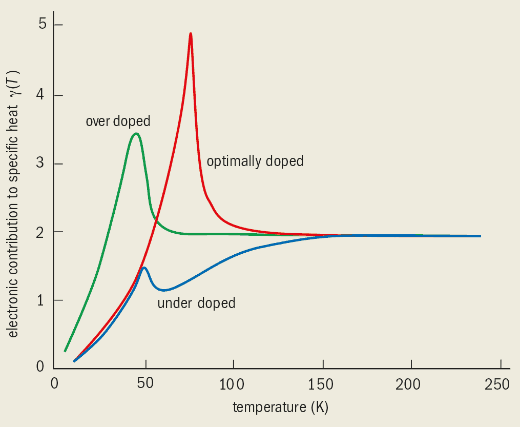
2 Indirect evidence for the pseudogap The electronic contribution to the specific heat capacity as a function of temperature for underdoped, optimally doped and overdoped samples of Y0.8Ca0.2Ba2Cu3O7–x. For optimally doped (red line) and overdoped (green line) samples the heat capacity remains constant as the temperature is lowered, then peaks at the superconducting transition temperature, Tc, and rapidly approaches zero in the superconducting state. For underdoped samples (blue line), however, the heat capacity starts to fall well above Tc as the temperature is reduced, and there is only a small peak at Tc. This is indirect evidence for a pseudogap. (J W Loram et al. 1997 Physica C282 1405)
When the quasiparticle approach is valid, there is a well defined boundary between particles and holes in both energy and momentum space at zero temperature. This boundary occurs at the Fermi energy and defines the “Fermi surface” in momentum space. However, the Landau quasiparticle model can only explain part of the phase diagram of the cuprates.
The best known characteristic of the superconducting region is the fact that the resistivity is zero. However, condensed-matter physicists measure many other properties of superconductors, such as the energy needed to split the Cooper pairs. This is the superconducting energy gap, 2D. The pairing process means that there are no single-particle excitations with energies of less than D in the superconducting state (hence the name gap).
Normal metals and Fermi liquids do not exhibit such gaps. Energy gaps show up clearly when the single-particle density of states is plotted – that is when the number of electronic states with a given energy is plotted as a function of energy. Energy gaps are also responsible for semiconductivity, but the mechanism that leads to the formation of the gap is completely different.
The part of the phase diagram between the underdoped and Fermi-liquid regions, and above the area with the highest superconducting transition temperatures, is called the non-Fermi-liquid region. The thermodynamic properties in this region are unexceptional and, within experimental uncertainties, are in fact similar to the behaviour of a Fermi liquid. However, this region is characterized by exceptionally simple but unusual power laws in all of its transport properties as a function of temperature. These transport properties include the resistivity, the optical conductivity, the electronic Raman-scattering intensity, the thermal conductivity, various nuclear relaxation rates, the Hall conductivity and the magnetoresistance. These unusual transport properties are why this part of the phase diagram is called the non-Fermi-liquid region.
The exceptional transport properties of the non-Fermi-liquid region led Phil Anderson of Princeton University to suggest in the late 1980s that radically new physics was – and still is – required to understand the cuprates. One of us and collaborators suggested that the non-Fermi-liquid region of the phase diagram is well described by the so-called marginal-Fermi-liquid hypothesis. Here the linewidth of a single-particle excitation is proportional to its energy, which means that the quasiparticles are not well defined, and there is no clear boundary between particles and holes at zero temperature.
This point was reinforced by angle-resolved photoemission spectroscopy measurements, which found no evidence for quasiparticles. On the other hand, the first derivative of the occupied density of states with respect to momentum is discontinuous, and this can be used to define a Fermi surface. But in the underdoped region, as we shall see, the concept of the Fermi surface itself is lost. For condensed-matter physicists this is very strange indeed.
Indirect evidence for the pseudogap region
A large number of experiments have probed the principal thermodynamic and transport properties of the underdoped region. The underdoped samples behave very differently from the overdoped and optimally doped ones (see Timusk and Statt in further reading).
For instance, the contribution of electrons to the specific heat divided by temperature, g(T), of the overdoped and optimally doped samples remains approximately constant as the temperature is reduced. At the superconducting transition temperature, Tc, this contribution peaks, before falling to zero as the sample is cooled further. For underdoped samples, however, g(T) starts to decrease with temperature well above Tc (figure 2). This may be taken as possible evidence for a “pseudogap” phase that exists above Tc and below a characteristic pseudogap temperature, Tp.
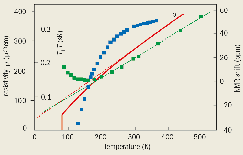
3 More indirect evidence for the pseudogap Signatures of the pseudogap in various transport properties for the underdoped compound YBa2Cu4O8. At high temperatures the resistivity (red solid line) decreases linearly with temperature, consistent with a non-Fermi-liquid behaviour (red dashed line). However, in the pseudogap region (i.e. below Tp) it drops faster with temperature, before falling to zero at the superconducting transition temperature (about 85 K). Similarly the NMR relaxation time (green squares) displays non-Fermi-liquid behaviour (green dashed line) before deviating at around 200 K. The NMR shift (blue squares) also deviates from the non-Fermi-liquid behaviour (not shown) below Tp. Note that the pseudogap expresses itself as a gradual change in behaviour as the sample is cooled and that the onset temperature is different for the different properties. (B Bucher et al. 1993 Phys. Rev. Lett.70 2021; H Yasuoka 1997 Hyperfine Interactions105 27; H Alloul et al. 1989 Phys. Rev. Lett.63 689)
For normal Fermi liquids the quantity S(T)/T – where the electronic entropy, S(T), is defined as S(T) = ò0Tg(T) dT – is proportional to the contribution of the conduction electrons to the uniform magnetic susceptibility, c(T). Both S(T)/T and c(T) have similar dependencies on temperature for a range of doping levels. In particular, the decreases in S(T)/T and c(T) in the pseudogap region are similar to each other, even though neither is that of a Fermi liquid. This implies that both the charge degrees of freedom and the spin degrees of freedom (which determine the magnetic properties) are suppressed. The simplest possibility, which is consistent with both the thermodynamic data and the photoemission experiments discussed below, is that the one-particle density of states is suppressed. Again, this is indirect evidence for a pseudogap.
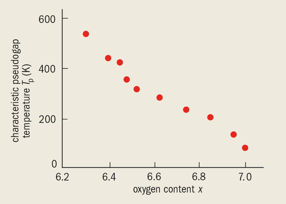
The pseudogap also manifests itself in various transport properties such as the resistivity, the nuclear magnetic resonance (NMR) relaxation time and the so-called Knight shift in NMR measurements. For instance, the cross-over from the linear dependence of the resistivity on temperature in the non-Fermi-liquid region to a stronger dependence in the pseudogap region is clear (figure 3). The characteristic temperature at which the influence of the pseudogap appears in a transport measurement depends on the property measured. It also depends systematically on the doping level (figure 4).
4 Doping and the pseudogap In addition to the characteristic pseudogap temperature, Tp, being different for different properties (figure 3), it also varies systematically with the level of doping, which is varied through the oxygen content in YBa2Cu3Ox. Tp is therefore a characteristic scale rather than an absolute temperature value. (Adapted from B Wuyts et al. 1996 Phys. Rev. B53 9418)
How big is the pseudogap?
Early evidence for the pseudogap in the underdoped phase came from indirect measurements like those described so far. What were really needed to explore and understand the pseudogap region were techniques that could directly measure the density of states. One of the best ways to do this is using angle-resolved photoemission spectroscopy (ARPES).
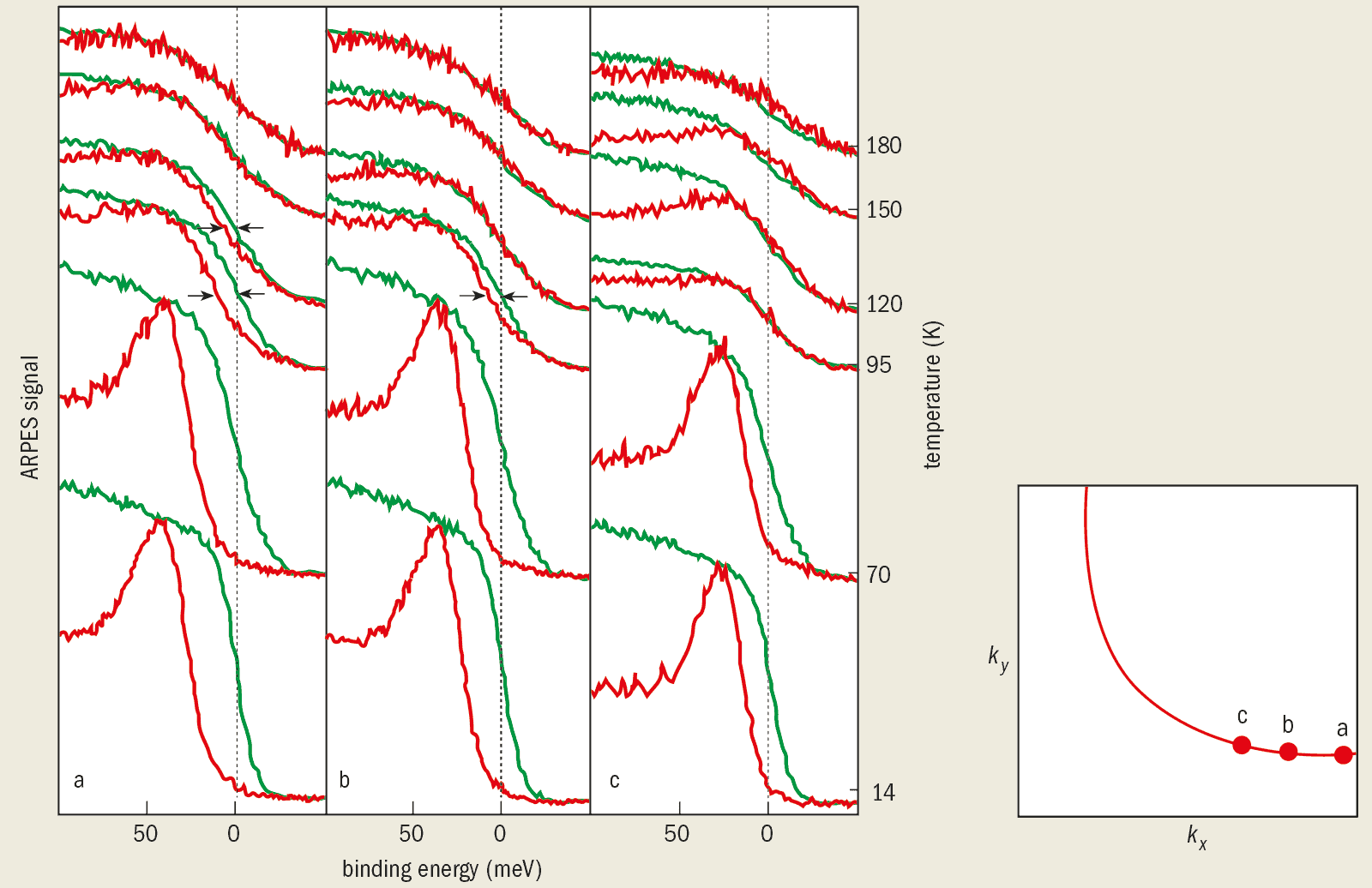
In a typical ARPES experiment, photons from a radiation source are directed at a sample. The photons have enough energy to expel electrons from the sample. If the direction and energy of the expelled electrons can be measured, it is possible to determine the momentum-dependent single-particle density of states below the Fermi energy. The pseudogap can be seen clearly in the ARPES data as a difference in the spectrum of the cuprate with respect to that of a normal metal (figure 5). Reassuringly, the pseudogap disappears above temperatures similar to those at which the transport properties change (figure 3). Moreover, this characteristic pseudogap temperature also changes with doping, similar to that seen in figure 4.
5 Direct evidence for the pseudogap Temperature dependence of the superconducting energy gap and the pseudogap for the underdoped compound Bi2Sr2CaCu2O8 at three different points on the ‘expected’ Fermi surface (marked a, b and c opposite) measured with angle-resolved photoemission spectroscopy (ARPES). The gap can be seen as the shift (to the left) of the leading edge of the spectrum (red lines) with respect to the reference spectrum of a normal metal (green lines). The spectra at the lowest temperature indicate that the magnitude of the superconducting gap is angle-dependent and they are consistent with d-wave symmetry being predominant. The superconducting energy gap persists as a pseudogap when the temperature is raised above the superconducting transition temperature for this sample (Tc=85 K). The ‘expected’ Fermi surface is determined from the Fermi surface near or above optimal doping: it is plotted in the plane defined by the momentum in the x- and y- directions in the copper-oxide planes. (J W Loram et al. 1997 Physica C282 1405)
On the Fermi surface, the size of the pseudogap also varies with the direction. In the plane defined by the momentum in the x and y directions in the copper-oxide planes, kx and ky, the pseudogap goes to zero in four directions (kx = ±ky). This four-fold pattern has the same symmetry as the energy gap in a d-wave superconductor. This could prove to be a useful clue to understanding the puzzling behaviour of the underdoped region.
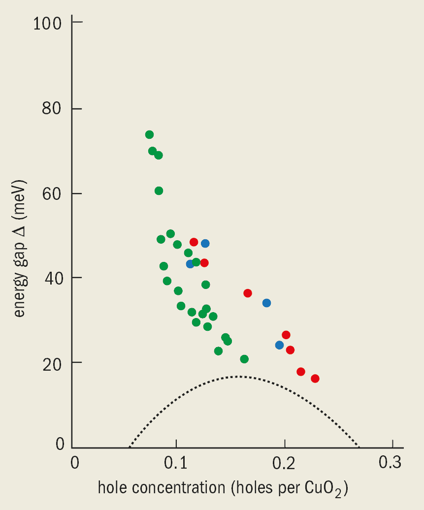
The characteristic energy of the pseudogap can be deduced from the specific-heat and ARPES data, and extrapolates to a value of about 100 meV at zero doping (figure 6). This is a surprisingly large value.
6 Surprising size of the pseudogap The energy gap determined by specific heat measurements (green), ARPES (blue) and tunnelling experiments (red) on YBCO (yttrium barium copper oxide) and BSCCO (bismuth strontium calcium copper oxide) samples. The gap is substantial: it is about 20 meV at optimal doping and extrapolates to about 100 meV at zero doping. The values measured by ARPES and tunnelling experiments agree with each other but seem higher than the specific heat values, which suggests that the former two techniques must also measure some multiple of the superconducting energy gap. The dashed line is 5kBTc(x). (J W Loram et al. 1997 Physics C282 1405)
The magnitude of the maximum gap varies with doping in a similar way to Tp. The ARPES signal is also continuous as a function of energy across the superconducting transition, which means that the pseudogap above Tc is as robust as the superconducting gap below Tc. Maybe there is nothing “pseudo” about this gap at all!
If the notion of a Fermi surface is used loosely (i.e. without paying attention to finite temperature effects), one might say that the Fermi surface in the pseudogap regions consists of four arcs the lengths of which progressively diminish as temperature is decreased. If the interpretation of the ARPES data in terms of Fermi arcs is taken literally, the implication is that in the region between the arcs, the distinction between electrons and holes is blurred. This is a very bizarre situation.
As mentioned above, the pseudogap extrapolates to a large value (about 100 meV) at zero doping. It is possible that the gap measured by ARPES below Tc is made up of the pseudogap, Dp(x), and some multiple of kTc(x). Indeed, the gap measured by ARPES seems to vary as ~[Dp(x)2 + m2kTc(x)2]-1/2 with m » 5. This suggests that the pseudogap might have a physical origin that is distinct from the superconducting gap.
Do we understand the pseudogap region?
The experimental discovery of the pseudogap phase in underdoped cuprates has presented a major challenge for theorists, who have responded with an impressive number of ideas.
Stripes. Some of these proposals rely on strong spin and/or charge fluctuations. Indeed, there is experimental evidence for “stripes” of charge and spin in several compounds in the underdoped phase. Two observations appear to challenge these proposals. First, no systematic correlations between the observation of stripes and either the characteristic pseudogap temperature, Tp(x), or the pseudogap energy, Dp(x), have been found. Second, the stripes appear not to produce the observed angular dependence of the pseudogap as seen using ARPES. It is also hard to see how stripes could lead to pseudogaps as large as those observed.
Antiferromagnetic fluctuations. The cuprates are antiferromagnets at low doping, so it is natural to propose that antiferromagnetic fluctuations are responsible for the pseudogap phase in the underdoped region (see Pines in further reading). This proposal faces similar questions as the stripes proposal regarding both the symmetry and the magnitude of the pseudogap.
Preformed pairs/superconducting fluctuations. Given that the symmetry of the pseudogap is the same as that of the superconducting state, it is natural to associate the pseudogap phase with fluctuations that lead to d-wave superconductivity. The pseudogap phase could result from the Cooper-pair formation energy being of the order of kTp(x), where k is the Boltzmann constant. These “pre-formed pairs” would cause all the thermodynamic and transport properties discussed above, and the single-particle spectra, to start changing around Tp(x).At least two versions of this idea have already been proposed. One version assumes that fluctuations in the phase of the superconducting order parameter (a complex number that describes the superconducting state) have such large amplitudes that they reduce the superconducting transition temperature from Tp to Tc (see Emery and Kivelson in further reading) This is supported by the small value of energy of these phase fluctuations in the cuprates. However, other measurements – notably measurements of high-frequency conductivity – appear not to support this idea (see Corson in further reading).
The second idea suggests that the coherence length (essentially the size of a Cooper pair) of the superconductors is so small that Cooper pairs form near Tp and that they all Bose condense into the same quantum state at Tc (see Randeria in further reading). However, experimental measurements of the coherence length do not support this.
Moreover, on the basis of either idea, one would expect the resistance in the pseudogap region to increase when an external magnetic field is applied, but this is not seen.
Spin-charge separation. Many theorists have developed models in which the spin and charge degrees of freedom associated with the holes become separated. The spins bind together to form so-called spin-singlets, and the energy needed to split them apart leads to the formation of a “spin gap”. The charge degrees of freedom, on the other hand, remain free. The spin-singlets are in a d-wave state that, according to these models, is a prelude to the d-wave superconducting state at low temperatures. An attractive feature of these models is that the characteristic spin-gap energy is the exchange energy, which in the undoped compound is of the order of ~100 meV. Indeed this value is similar to the characteristic energy of the pseudogap extrapolated to zero doping.Many different versions of this idea, which was first proposed by Phil Anderson, have been pursued as experiments (see Lee in further reading). However, the fact that the specific heat (which is related to all the excitations) and the magnetic susceptibility (which is related to the spin excitations) behave in a similar fashion in the pseudogap region poses a problem for this approach. Also, the theory still has to explain the remarkably simple power laws observed in the transport properties and the single-particle spectra measured in the non-Fermi-liquid region of the phase diagram.
Quantum critical points. This set of theories involves a point in the phase diagram where the transition temperature goes to zero as a function of some parameter, such as doping, pressure or the strength of an applied field – a so-called “quantum critical point” (see Sachdev in further reading). The transition must be between a phase with order or symmetry and one without such order. In other words it must involve a broken symmetry.The marginal-Fermi-liquid nature observed in the non-Fermi-liquid region of the phase diagram is consistent with a quantum critical point close to optimal doping. Several questions arise in applying this model to the cuprates. What is the broken symmetry associated with the pseudogap phase? And why are the thermodynamic properties at Tp(x) not singular, as often happens at such transitions?
One possibility, suggested by one of us (see Varma in further reading), is that the broken symmetry is a very elusive order parameter in the pseudogap region, and that there is a quantum critical point at the transition between the pseudogap and non-Fermi-liquid regimes. In this broken symmetry each unit cell breaks up into four “plaquettes” in which circulating currents flow between the copper and oxygen ions in consecutively opposite directions. Both time-reversal and four-fold rotational symmetry are broken by these currents, while the product of these two symmetries is preserved, as is translational symmetry.
This model makes predictions for the single-particle spectra, and also for the transport, magnetic and thermodynamic properties. However, only a direct observation of the proposed symmetry breaking – in, for example, an ARPES experiment with circularly polarized light – will make this exotic idea credible.
Where next?
Looking at the phase diagram for the cuprates (figure 1), it would be surprising if the four major regions – the pseudogap, the non-Fermi-liquid, the Fermi liquid and the superconducting regions – were not related. The understanding of the underdoped/pseudogap region may well hold the key to the understanding of the physics of the cuprates and, in turn, high-temperature superconductivity.
Given the large energy associated with the pseudogap, we would expect that the low-energy excitations would have unusual wavefunctions. So far experiments have concentrated on the energetics of these materials. However, this is not enough to distinguish between the many different models of high-temperature superconductivity that have been proposed. There is a clear need for experiments that can provide information about the wavefunctions (which could be provided by measurements of various correlation functions).
Of course, it could be that these experiments eliminate all of the theories, in which case it will be back to the drawing board for the theorists.
The 0.5 nm nanotube was made by boring a hole into a graphite rod. The hole was then filled with cobalt metal powder – which acts as a catalyst – and a mixture of nanotubes and other carbon-based material. A high-voltage electric arc was then applied to the graphite rod generating an carbon plasma from which the nanotubes were produced. The team believe that the nanotubes grow from curved carbon fragments in the rod. The diameter of the nanotube was measured with a high-resolution electron microscope. The 0.5 nm diameter nanotube was the innermost shell in a multiwall nanotube. It is not yet clear if such small tubes can occur as single-wall nanotubes.
The smallest nanotube previously reported had a diameter of 0.7 nm, which is the same as the diameter of a carbon-60 molecule. Since carbon-36 and carbon-60 molecules have any different properties, the researchers speculate that the new nanotubes may have “many unusual properties.”
White Mars is about a group of men and women who are marooned on Mars at the end of the 21st century. Living in enormous self-perpetuating domes, they produce their own food and oxygen, and extract water from the planet’s core. On this austere Martian world, members of the colony set out to create a Utopian society. The book examines whether such a society could be created and whether humans can achieve a better world and a happier future.
It was a chance encounter that brought the authors together. Aldiss, who has written over 20 novels, had decided to sell his house near Oxford. Penrose, who is based at Oxford University, was also planning to move and was shown Aldiss’ property by his estate agent. He eventually bought Aldiss’ home, and the two writers became friends as negotiations proceeded.
One night, Aldiss had a vivid dream about a group of people living on Mars. “I woke up, immediately wrote down what I had dreamt and then approached Roger and told him my story,” he explains. “Roger thought it was a great idea, and was very keen to get involved in writing a book. My dream that night forms the crux of the book.”
Luckily for Aldiss, Penrose is something of a science-fiction fan, citing Isaac Asimov, Arthur C Clarke and John Wyndham as particular favourites. “I had felt for some time that I might like to have a go at science fiction and then – rather fortuitously – this collaboration with Brian came along,” explains Penrose. “The idea of a book about a Utopian society might sound boring and starry-eyed, but I don’t think it’s turned out like that.”
So how did the two authors collaborate in practice? “It’s hard to say exactly what happened because it all took so long,” recalls Aldiss. “Like a marriage, it was a mystery even to the parties involved.” However, Aldiss reveals that the bulk of chapter 11, which he says contains most of the hard science, is by Penrose. “But Roger has always been a really bold thinker and he made big contributions elsewhere.”
Penrose is more modest. “Basically, Brian did all the writing and I would add bits of dialogue to help explain some of the science, although I also produced some ideas that significantly altered the plot,” he says. “It was certainly different from what I normally do and gave me the opportunity to explore the implication of some crazy scientific ideas.”
One problem for Penrose was that some of the science-fictional ideas came rather close to his own. “I wanted to differentiate between the two and make sure that our currently accepted scientific knowledge is used correctly in the book.” One way that he does this is through a character called Thorgeson, who explores the “conventional” ideas of physicists at the time. “The irony is that Thorgeson expresses ideas on consciousness that are not dissimilar from my own. While my ideas are currently regarded as unconventional, in the story they are presented as outdated.”
So does Penrose have any plans for further science-fiction books? “Yes, I think I’d like to do some more, but whether on my own or with Brian I’m not sure. It’s just a question of finding the time.”