Researchers in the US have developed a rapid, artificial intelligence (AI)-based test that can identify patients with an abnormal heart rhythm, even when it appears normal. This 10 second test for atrial fibrillation could be a significant improvement over current test procedures that can take weeks or even years (Lancet 10.1016/S0140-6736(19)31721-0).
Atrial fibrillation is a common cardiac condition that is estimated to affect between three and six million people in the US alone. The condition is associated with an increased risk of stroke, heart failure and mortality – but it is underdiagnosed. This is because it can be asymptomatic and the patient’s heart can go in and out of the arrhythmia, making diagnosis tricky. It is sometimes caught on an electrocardiograph (ECG), but often detection requires the use of implantable or wearable monitors to capture infrequent atrial fibrillation episodes over time.
“Atrial fibrillation is an arrhythmia where the atrium, or top chamber of the heart, loses its coordinated contractual activity and instead quivers, because the electrical impulse is changed in the way it courses through the atrium,” explains Peter Noseworthy of the Mayo Clinic. “So, the top chamber beats irregularly and it causes the bottom chamber, the ventricle, usually to beat fast and irregularly, which can be bothersome, but most importantly it predisposes people to risk of stroke.”
He adds that atrial fibrillation can be caused by many conditions, such as valvular heart disease, sleep apnoea and hypertension, but often doesn’t have a clear underlying cause.
To develop a low-cost and noninvasive test for atrial fibrillation, Noseworthy and colleagues trained and tested an AI model using data from nearly 650,000 ECGs from over 181,000 patients who attended the Mayo Clinic between December 1993 and July 2017. While some of the patients were known to have atrial fibrillation, they all had at least one 10 s ECG showing a normal heart rhythm.
Noseworthy tells Physics World that researchers suspect that atrial fibrillation usually happens in a heart that is somehow abnormal. The team hoped that this would leave a signature that could be detected on an ECG during normal heart rhythm.
The researchers trained the AI model using data from 70% of the patients, validated the model using data from 10% of the patients and tested it on data from the remaining 20%.
They found that the AI was able to detect differences in the ECGs of patients with atrial fibrillation. From a single 10 s ECG scan that appeared to a medical professional to show a normal heart rhythm, the AI was able to identify patients with atrial fibrillation with an accuracy of 79%. When multiple ECGs for the same patient were tested, the accuracy improved to 83%.
“When we look at the ECGs, they don’t have a single pattern to them, but the AI is able to identify many different, more subtle patterns that we may as cardiologists just recognise as mild abnormalities and do not really draw any attention to,” Noseworthy explains.
According to Noseworthy, the test has two main potential applications: pre-screening the general population to identify those who could benefit from long-term screening for atrial fibrillation; and testing patients who have had a stroke to identify those who could benefit from an anticoagulant or longer term screening with an implantable device.
These possibilities need to be explored further and the AI tested on other datasets and the general population, Noseworthy says. “Everybody in our dataset came to medical care and had an ECG, so it is going to be enriched with people who had some sort of cardiac issue or are concerned about a cardiac issue,” he explains.
In a linked comment, Jeroen Hendriks of the University of Adelaide in Australia says that this approach could lead to a paradigm shift in recording normal rhythm rather than atrial fibrillation on an ECG, with a “specific focus on identifying structural changes”. He cautions, however, that the AI network “has been tested to retrospectively identify atrial fibrillation rather than predicting atrial fibrillation”, stating that it needs further validation.
Hendriks concludes that the researchers “are to be congratulated for their innovative approach and the thorough development and local validation of the AI enabled ECG. Given that AI algorithms have recently reached cardiologist level in diagnostic performance, this AI-ECG interpretation is ground-breaking in creating an algorithm to reveal the likelihood of atrial fibrillation in ECGs showing [normal] rhythm”.
From the Huygens pendulum clocks in the seventeenth century onwards, the synchronization of coupled oscillators has had numerous practical uses. While most of these applications have been in mechanical and electrical engineering, nowadays there is increasing focus on applications in biology and neuroscience. With the development of nanotechnologies, scientists’ efforts have centred on synchronizing oscillatory nanoelectromechanical systems (NEMS), for applications such as on-chip time keeping, and mass, gas, and force sensors.
Martín Colombano and Guillermo Arregui from the ICN2 Phononic and Photonic Nanostructures Group in Barcelona and Universitat Autònoma de Barcelona, alongside colleagues in Spain and Italy, achieved spontaneous synchronization of coherent mechanical motion of a pair of one-dimensional silicon optomechanical cavities (OMC) integrated in the same chip, by a weak interaction between the two mechanically linked cavities. The results pave the way towards synchronizing arrays of nanoscale mechanical oscillators, building networks that may be useful in neuromorphic computing.
Self-sufficient yet sensitive
To enable spontaneous synchronization between two dynamical systems, they must firstly be self-sustained oscillators, that is, they must maintain the same rhythm, with no explicit time dependence, and their oscillation should be determined by the parameters of the system and stable to small perturbations. In addition a weak interaction should be able to adjust the rhythm of the oscillators within a certain range of mismatch of the systems. The experiment by Colombano, Arregui and colleagues is the first to fulfill these conditions for nanoscale OMCs.
In the experiment, the researchers optically isolate the OMCs from each other, measure them independently, driving each one to a state of high amplitude, coherent, and self-sustained mechanical motion using the radiation pressure force exerted by two infrared lasers. They named the two cavities master and slave, where the cavity displaying the higher oscillation frequency and longer optical resonance wavelengths is the master and the other is the slave. The master oscillation amplitude is significantly larger, which tells us that its dynamics are much less sensitive to slave oscillations. Nonetheless, the master is mechanically excited by coherent motion of the slave through mechanical coupling of both OMCs.
The research also explores the effect of the top heating laser illuminating the master cavity. When this laser is switched on, the synchronized state is lost and the coupling is reduced. When the laser is switched off, it takes several microseconds for the OMCs to reach the synchronized state. This demonstrated dynamical switching between the two states by an external heating source.
A wave-damping scheme that draws on the principles behind the much vaunted “invisibility shields” made from metamaterials could calm the waters for boats moored in harbours and ports. The team who came up with the idea have demonstrated that it works in a large wave tank, and hope soon to put it into practice on the coast of China.
The method involves manipulating water waves so that their amplitude falls to almost zero within narrow channels such as the spaces between jetties or wharves in a dock. Devised by civil engineer Zhenyu Wang of Zhejiang University in Hangzhou, physicist Huanyang Chen of Xiamen University, and their coworkers, it exploits principles originally applied in optics to shape and guide electromagnetic waves.
The general idea is that, by varying the refractive index in different regions of a transparent material, light waves passing through it can be locally enhanced or suppressed in ways that needn’t follow the normal laws of optics. Using materials with spatially varying refractive index – a measure of the propagation speed of electromagnetic waves – researchers have shown how to make “invisible” cloaking devices and other optical structures at the wavelengths of visible light.
The approach relies on classical wavelike behaviour, and so the same mathematical principles can be used to control and direct other kinds of waves. It has already been applied previously to acoustic waves, water waves and even seismic waves, raising the prospect of making cloaks that shield buildings or whole cities from earthquakes.
Redirecting wave energy
The ability to control sea waves has obvious potential in marine engineering. Wave suppression, for example, could reduce coastal erosion and drag on ships, while focusing ocean waves could be valuable for energy generation. But although such ideas have been explored theoretically, relatively little has been done to test them experimentally.
That’s where Wang’s team comes in. At Zhejiang University they have a large water tank, 60 m long by 1.2 m wide, for simulating the marine environment. Wang has teamed up with theorist Chen, who has worked previously on using transformation optics to devise new types of lens, light concentrators and other structures. Having moved from inland Suzhou University to coastal Xiamen, one of China’s major ports, Chen has become attuned to the possibilities of the theory for marine applications.
Wang explains that rather than trying to block or resist ocean waves using breakwaters, as in conventional approaches for protecting harbours, they redirect the wave energy. “Our new way of thinking is to defuse and manipulate water waves,” he says.
The team has designed a water-wave damping structure simple enough to be implemented cheaply in real-world settings. The idea is straightforward: for water waves, the equivalent of a refractive index can be simply the water depth. To manipulate waves one then needs only to place a structure on the seabed that makes the water locally shallower.
However, to get the optimal effect this depth must be altered with a smooth and carefully shaped gradient. The researchers calculated that submerged batons with gently rounded ends either side of a water channel could concentrate the energy of an incoming plane wave within the regions above the batons themselves, leaving the centre of the channel calm. “By arranging the refractive index profile, we can squeeze the waves along the two sides of the channel and create a cloaking region [in the middle],” says Chen.
Putting it to the test
Their tests in the wave tank, using batons 6 m long and 15 cm wide placed against the two edges, confirm the idea. A toy boat placed in the channel centre in water about 16–18 cm deep looks more or less immobile to the naked eye as waves of frequencies of around 0.6–0.9 Hz and heights of around 1 mm enter the “shielded” region. But when floating directly over the submerged batons, the boat bobs up and down visibly with an amplitude of up to 6 mm. The cloaking will work for a wide range of wave frequencies.
“For a real port location, we know the most frequently occurring period and wavelength of water waves,” says Wang. “Then we can design the gradient water depth and the corresponding underwater structure accordingly”. He thinks that the method might be most easily applied to yacht docks, and the team is now hoping to try out the idea in Xiamen or the Zhoushan archipelago in Hangzhou Bay, where Zhejiang University has an island with a facility for running experiments under ocean conditions.
Wave suppression “is an important goal for port and harbour applications”, says physicist Léo-Paul Euvé of ESPCI in Paris, “and I think this system could be applied in a real-world setting.” Currently ports tend to use large dikes or barriers to block waves, he says, and a system like this “could be an interesting alternative”. He adds that by concentrating the wave amplitude in a small area, the design “could be also interesting for extracting wave energy”.
This is “beautiful physics” says Che Ting Chan of the Hong Kong University of Science and Technology, an expert on optical and acoustic metamaterials. But he stresses that “the experiments are carried out in a highly controlled environment, and the real world is way more complicated” – for example because of issues like nonlinearity of the waves, viscosity, turbulence, and irregularities on the bottom surface of a channel. So he says that, although the method “might be useful in calm harbours or channels, I wouldn’t dare to recommend its use to taming hurricane or tsunami waves, which are very nonlinear and violent.” Chen agrees: “Tsunamis will not be easy to handle, and nonlinear effects would need to be considered [for that]”, he says.
A new toolbox for sophisticated quantum simulators, in which qubits can directly communicate through so-called “topological radio channels”, has been proposed by physicists in Germany and Spain. Researchers led by Alejandro González-Tudela at the Max Planck Institute for Quantum Optics in Garching constructed the theory by transferring the principles of topology from condensed matter to photonics.
Topology has become an incredibly influential branch of mathematics in recent years. In geometric terms, it describes how an object can easily be transformed into another object with the same number of holes, without cutting or gluing. In condensed matter, meanwhile, topological materials display similar geometries on the molecular scale, which gives them diverse mechanical and electrical properties.
Recent studies have explored how the principles of topology can be transferred from condensed matter to photonics, potentially allowing researchers to induce exotic properties of light by engineering topological materials. In this new study, González-Tudela’s team – which included physicists at the Institute of Materials Science of Madrid – showed that a variety of unprecedented quantum optical phenomena can emerge when these topological photonic systems are coupled to quantum emitters.
The researchers started by describing a simple model in which a line of photon-emitting qubits is coupled to a one-dimensional topological photonic waveguide, and the emission frequency of one qubit lies in the energy gap where no electron states can exist in the solid. In this situation, the bound state of the qubit becomes chiral, meaning it can only be located on either the left or right side of the emitter. The end result is that information can only flow in one direction, leaving the other direction completely dark.
From this model, González-Tudela and colleagues propose a toolbox for allowing two specific, distant qubits to communicate with each other through a so-called topological radio channel. By tuning the topology of the waveguide to induce specific chiral bound states, particular pairs of qubits could be consciously chosen to interact with each other on these different channels.
This principle addresses a key challenge for quantum simulations: how to account for specific interactions within highly complex many-body systems. Using current simulation techniques, such as ultracold atoms trapped by an optical lattice, it is incredibly difficult to direct the flow of information between emitters.
The toolbox proposed by the team could allow for significant improvements to these techniques, providing a way to account for the intricate webs of long-range interactions between qubits. With further research into how their ideas can be implemented, González-Tudela and colleagues hope that the technique could help to explore the diverse behaviours of quantum many-body systems in unprecedented detail.
Situated around 800 km from the North Pole, Eureka is one of the coldest inhabited places in the world. With a mean annual air temperature of -19.7° C and polar night lasting from mid-October until the end of February, this Arctic weather station on Ellesmere Island has just a handful of residents. Now research shows that climate change is biting even here.
Ellesmere and Axel Heiberg Islands are the two most northerly islands in the Canadian high Arctic. Permafrost here is over half a kilometre thick and has a mean annual temperature of -16.5°C at its surface. It’s been this way for thousands of years; people assumed that the cold temperatures would keep permafrost in the region safe.
Wayne Pollard from McGill University, Canada, has monitored this permafrost since 1989, flying the same transect from the Eureka Weather Station by helicopter every summer. He scans the landscape beneath for the tell-tale features where permafrost thaw has made horseshoe-shaped “bites” known as retrogressive thaw slumps.
Until 2003 Pollard generally spotted somewhere between 50 and 100 slump features every summer. Since then numbers have increased; on three occasions there have been over 200 slumps each year.
Pollard used GPS measurements and satellite imagery to measure the rate of headwall retreat for some of the more recent slumps, working with colleagues from McGill University and University of Alaska Fairbanks, US. These features are growing fast, the team found, at up to 26 m per year.
“These are dramatic landforms as they appear suddenly and grow quickly,” says Melissa Ward Jones of McGill University. “The land surface lowers as ground ice melts and releases large volumes of sediments that get displaced downslope and can enter water bodies and impact aquatic ecosystems. They also impact terrestrial ecosystems because often vegetation that grows after the disturbance is different.”
Comparing slump frequency with average July temperatures suggests that recent record summer warmth – with average air temperatures of 7 °C or more – has been a trigger. “The widespread increases [in slumps] we’ve seen in the last 16 years is likely attributed to increases in summer air temperatures,” says Ward Jones.
These exceptionally warm summers appear to have driven permafrost thaw despite average annual temperatures remaining fairly steady over time.
“I think we should approach these high Arctic observations as a warning sign to changes that will be experienced in southern areas, because an area we think of as being really cold and stable is undergoing rapid change,” says Ward Jones.
What are the most common clinical applications for 3D-printed models created from MRI scans of paediatric patients? A team from Ohio explored the various applications and the role radiologists play in production of the models in a new article, recently published online in the Journal of Magnetic Resonance Imaging.
“We wanted to investigate 3D printing with MRI because most applications using the technology have used CT scans in the past,” first author Jayanthi Parthasarathy told AuntMinnie.com. Parthasarathy is manager of 3D printing at Nationwide Children’s Hospital‘s department of radiology in Columbus, OH.
“In children, you also want to avoid radiation as much as possible,” she said. “So our goal was to see what were the most common applications in the paediatric world for 3D printing with MRI, and if it could give us the same benefits as 3D printing with CT does.”
To that end, the group surveyed all 3D printing articles that were listed in the PubMed database from 1990 to 2019. They found 92 publications focused on paediatric 3D printing based on MRI scans as of March 2019. The vast majority of the articles were published in the last five years, with a peak of 19 articles published in 2017 (J. Magn. Reson. Imaging 10.1002/jmri.26870).
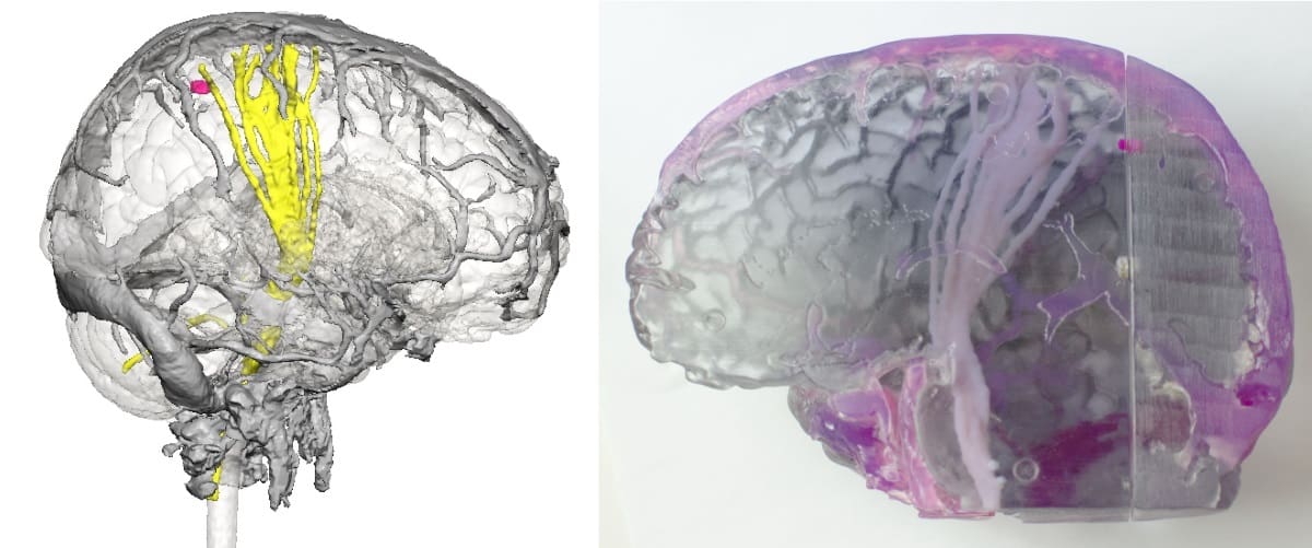
A virtual 3D model based on brain MR images (left). A patient-specific 3D-printed brain (right). (Courtesy: Jayanthi Parthasarathy)
The researchers for these prior studies most frequently used 3D-printed models for cardiovascular applications (35%), followed by use in neurosurgery (14%), education and training (13%), imaging (8%) and urology (8%), among others. Parthasarathy and colleagues discussed the specifics of several of these applications in their review:
Cardiology: 3D-printed models based on MR angiography images primarily serve to improve clinicians’ understanding of the unique and complex arrangement of patient vasculature, which has proved critical for presurgical planning, the authors noted. The enhanced, tangible visualization of young patients’ hearts has proved especially valuable in the management of congenital heart disease and for simulating interventional cardiology procedures.
Neurosurgery: Neurologists and neurosurgeons have used 3D-printed brain models as an adjunct during surgical planning for sensitive conditions such as intractable epilepsy. The models can display the entirety of the nerve tract in the brain (fusing multiple MRI contrasts in a single print), which has allowed for realistic, cost-effective simulation of challenging surgeries, according to the researchers.
Education and training: Beyond surgical planning, 3D-printed models have also helped medical staff and patients and their family members come to understand anatomy more readily than by examining conventional medical imaging and even virtual 3D models.
Imaging: Various groups have additionally used 3D printing technology to determine the best imaging sequences for MRI protocols.
Urology: A number of investigators have demonstrated 3D-printed urologic cancer models to facilitate preoperative planning as well as improve patients’ understanding of their condition.
The wide range of MRI-based 3D printing applications for paediatric cases has largely depended on collaborations between hospitals and external 3D printing services that necessitate long processing times, Parthasarathy said. However, point-of-care manufacturing for 3D-printed anatomical models, often led by radiology departments, has become increasingly common in recent years.
Better imaging techniques, demonstrated benefits of the enhanced visualization provided to surgeons and patients before surgery, availability of low-cost printers, and new 3D printing materials that better resemble human tissue have all contributed to this trend, and “new reimbursement pathways will add to a multifold increase in the utilization of the technology,” she said.
“Radiologists are the people who do all of the imaging, and, as of now, the 3D printing applications at most hospitals are started in the radiology department,” Parthasarathy said. “In a sense, the radiologist is the person who is the brains behind all of this. And in fact, radiology has taken up 3D printing in a big way.”
If the Starship Enterprise dipped into the Earth’s atmosphere at a sub-warp speed, would we see it? And if the craft were visible, would it look like the object we’re familiar with from TV, with its saucer section and two nacelles? Well, if the Enterprise were travelling fast enough, then – bright physicists that we are – we’d expect the craft to experience the length contraction dictated by special relativity.
According to this famous principle, a body moving relative to an observer will appear slightly shorter in the direction the body’s travelling in. Specifically, its observed length will have been reduced by the Lorentz factor (1–v2/c2)1/2, where v is the relative velocity of the moving object and c is the speed of light in a vacuum. However, the Enterprise won’t be seen as shorter despite zipping along so fast. In fact, it will appear to be the same length, but rotated.
You might not have heard of this phenomenon before, but it’s often called the “Terrell effect” or “Terrell rotation”. It’s named after James Terrell – a physicist at the Los Alamos National Laboratory in the US, who first came up with the idea in 1957. The apparent rotation of an object moving near the speed of light is, in essence, a consequence of the time it takes light rays to travel from various points on the moving body to an observer’s eyes.
Terrell’s insight was that even if those rays leave different parts of the moving body at the same time, they won’t reach the observer’s eyes at the same time. The net result is a distorted view. Amazingly, for an object that subtends a small solid angle, the Terrell effect will cancel out the Lorentz contraction, making the object appear to have been rotated. Indeed, it allows you to see partly around the object and observe its reverse side.
Of course, the rapidly moving Enterprise would also be subject to the Doppler effect, which would render it a different colour. Indeed, the frequency shift might even make the craft totally invisible to human eyes. The Enterprise would also appear brighter or dimmer due to relativity’s “headlight effect” (which I’ll come back to later). All in all, these effects will make a rapidly moving object, such as the Enterprise, appear nothing like it does at rest.
Now, if you think that’s confusing – don’t worry, you’re not alone.
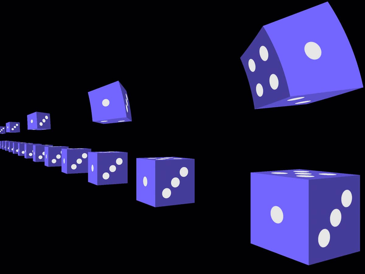
Curiouser and curiouser: A row of stationary dice (bottom), with other dice moving from left to right (top) at 90% of the speed of light. (Courtesy: CC BY-SA 2.0-de/Ute Kraus)
Length contraction: the short story
The idea of length contraction was postulated by the Irish theoretical physicist George FitzGerald in 1889 and by the Dutch theorist Hendrik Lorentz in 1892. Also known as Lorentz–Fitzgerald contraction or just Lorentz contraction, it was invoked to account for the negative outcome of Albert Michelson and Edward Morley’s memorable experiment of 1887. The two Americans had famously tried – and failed – to detect the “aether”, a hypothetical stationary medium that was supposed to carry electromagnetic waves, much as the surface of water carries water waves.
Keen to rescue the hypothesis of a stationary aether, Lorentz and Fitzgerald’s solution to Michelson and Morley’s null result was to suggest that objects travelling at a substantial fraction of the speed of light will – when viewed by another observer – appear shortened in the direction of their travel. Based on a calculation by Oliver Heaviside of how the magnetic vector potential in Maxwell’s equation transformed between reference frames, their idea was, in truth, just one of a few proposed “solutions”. None was completely satisfactory, however, and for many years, length contraction remained an ad hoc hypothesis.
It was only in 1905 that Albert Einstein cut through the confusion when he published his special theory of relativity. It did away with the aether altogether and proposed two postulates. The first is that the laws of nature are the same in all “inertial” reference frames – i.e. those frames moving at a constant velocity with respect to one another, in which any object with no net forces on it will appear at rest. The second postulate states that an observer in any inertial reference frame will measure the speed of light in a vacuum to be the same.
From his theory, Einstein derived length contraction as well as time dilation, the equivalence of mass and energy, and more. In particular, he realized that an observer at rest on a high-speed train will measure the length of a passing high-speed train as shortened in the direction of its motion, by the factor (1–v2/c2)1/2 where v is the relative velocity between the observer and the other train. (Paradoxically, an observer on that train will measure the first as shortened by the same factor. Isn’t special relativity fun?)
Length contraction has never been directly measured. But its effects show up in the magnetic force that acts between parallel, current-carrying wires. Bizarrely, this force, which is purely magnetostatic, appears in one wire due to length contraction as experienced by the charge carriers in the other wire’s frame. (It’s complicated. You can find more information in two papers by Paul van Kampen from Dublin City University – Eur. J. Phys29 879 and Eur. J. Phys31 L29 – and also in the chapter “Current-carrying wires and special relativity” in the book Trends in Electromagnetism). Current-carrying wires aside, there is little doubt that Lorentz contraction occurs if length is measured – that is, when different points on a moving object are all measured at the same instant of time in the observer’s stationary frame of reference.
But when you view an object with your eyes or a camera, it’s a different story. You’re then recording the photons the object emits – and these photons arrive at your eyeball or camera lens at the same time. What both Einstein and Lorentz overlooked, however, is the fact that the photons may have been emitted by the object at a different time, especially if the object is large. In fact, in 1922 Lorentz erroneously claimed, in the Dutch version of his Lectures of Theoretical Physics, that the contraction could be photographed.
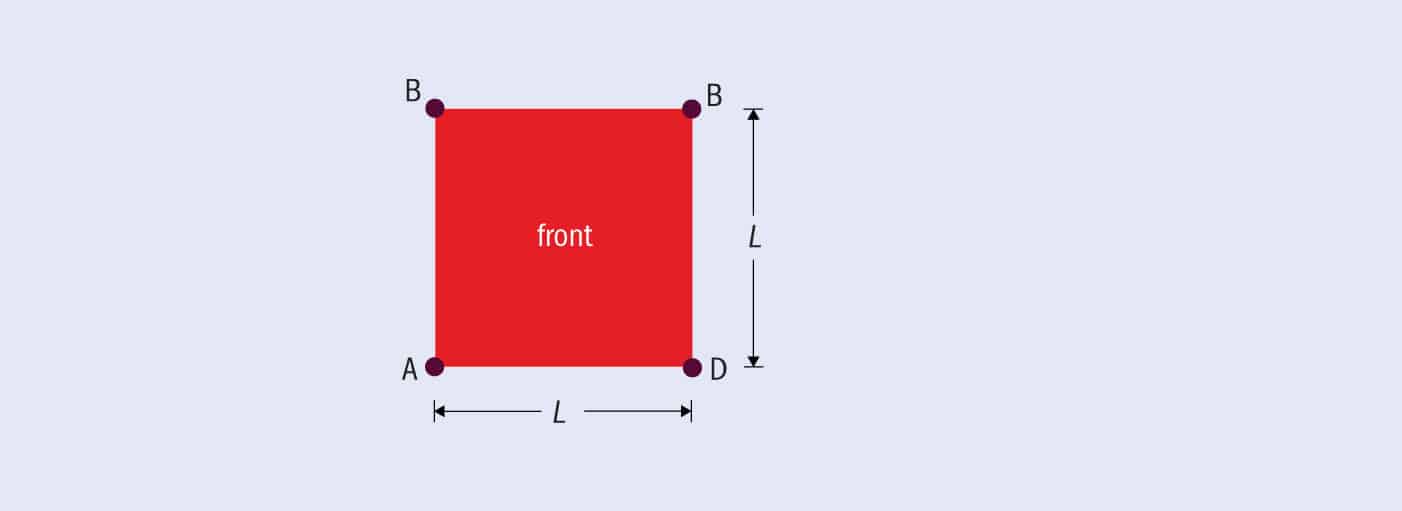
1 Why Lorentz contraction disappears for a cube moving at near the speed of light
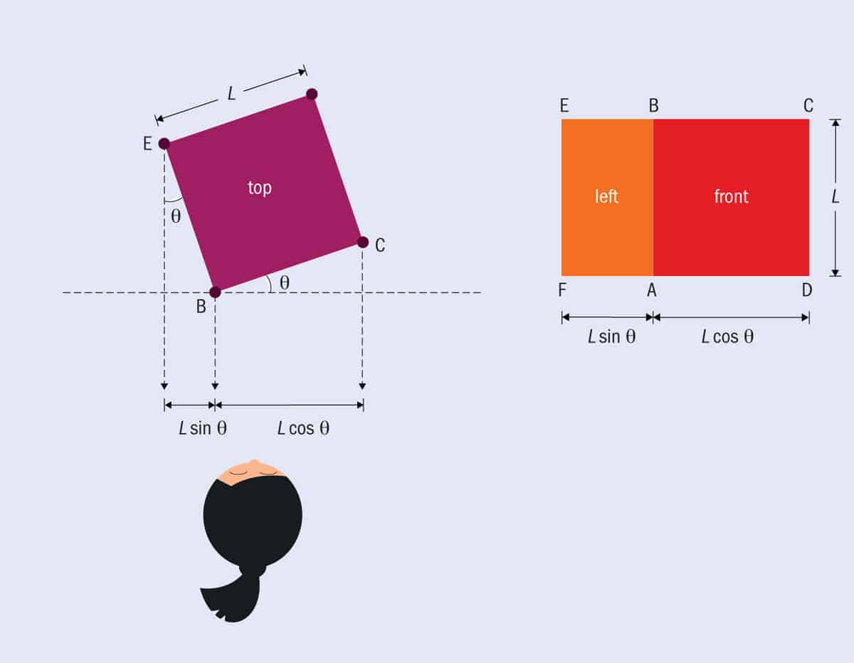
(a) To understand why an object appears rotated, not contracted, when moving at relativistic speeds, imagine you’re looking at a cube of length L moving from left to right. You, the observer, are standing far enough away, compared to the cube’s dimensions, that the solid angle subtended by the cube is small and light rays from it are essentially parallel.
(b) If the cube is moving much more slowly than the speed of light, all you’d see – when the object’s directly in front of you – would be the cube’s “front” side.
(c) Now consider a cube at rest or moving slowly, but rotated around an axis through the top and bottom by some angle relative to the line of sight. For an observer looking head-on, two sides would now be visible but not seen to be of equal area.
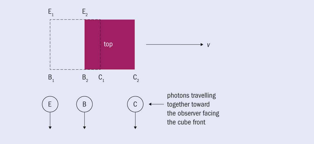
(d) If an unrotated cube is moving at a substantial fraction of the speed of light, but without considering special relativity, there is no length contraction in any direction…
(e) Continuing from above, but still not considering special relativity, the observer will not only see the “front” of the cube but, due to the “retarded” photons, also its “left” side, with its length L reduced to L(v/c). The cube will appear distorted – though not rotated, since the “front” is not foreshortened and still has a length L.
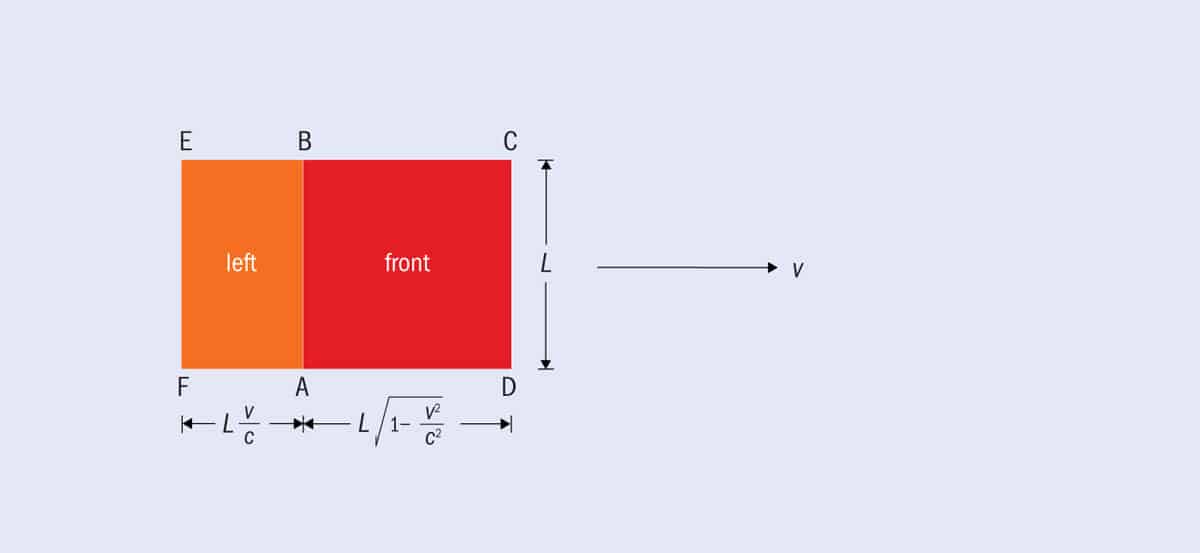
(f) Finally, let’s consider both photon retardation and relativistic effects, as we must in the real world. Moving at near the speed of light, the “front” of the cube is foreshortened and appears to have a length L(1–v2/c2)1/2. Compared to part b, the cube appears the same as one of length L but rotated by an angle θ, where (as in part c) cosθ = L(1–v2/c2)1/2 /L i.e. θ = arcsin(v/c). The moving cube will thus look the same as an undistorted, rotated, non-relativistic cube of length L. The Lorentz contraction has amazingly “disappeared”.
Lost in history
Over the years, few people paid much attention to observing Lorentz contraction. Anton Lampa, an Austrian physicist who had once helped Einstein get his first university professorship, did publish a paper on this topic in 1924 (Zeitschrift für Physik 27 138). Concerning the appearance of a moving rod to an observer, his work was unfortunately largely overlooked. Indeed, in his famous 1940 children’s book Mr Tompkins in Wonderland, the Russian-born physicist George Gamow got length contraction all wrong. He showed bicycles as simply shortened in the direction they are travelling, instead of being distorted and elongated when approaching an observer, or contracting as they receded into the distance.
Researchers only properly started to take notice of the practicalities of observing Lorentz contraction when Terrell published an internal Los Alamos article in 1957 about the effect, followed two years later by a paper in the Physical Review (116 4). His work was spotted by the theorist Victor Weisskopf, who, while serving as president of the American Physical Society, wrote an article for Physics Today presenting Terrell’s findings in a simpler form.
Like Terrell, Weisskopf also noted an earlier 1959 article by the British mathematical physicist Roger Penrose, in which he analysed the appearance of a relativistically moving sphere. In his 1905 paper on special relativity, Einstein had said that such a sphere would look like an ellipsoid, contracted in the direction of motion. But Penrose reckoned that the object would still be spherical, albeit rotated. Indeed, thanks to Penrose’s insights, the Terrell effect is sometimes referred to as the “Penrose–Terrell effect” (though the two worked independently).
Terrell’s and Penrose’s simple insight – overlooked by nearly every physicist before them – was that light rays that simultaneously leave a moving object do not necessarily strike the eye or camera film at the same time. The eye or lens sees images from photons that strike it simultaneously, but these photons – especially for a rapidly moving object – do not leave the object simultaneously. Surprisingly enough, in certain circumstances this difference exactly cancels the Lorentz length contraction and the moving object appears rotated.
Rotation, not contraction
To appreciate why Lorentz contraction disappears for an object moving at relativistic speeds, Peter Signell from Michigan State University has considered the simple case of a cube moving left to right when viewed head-on (see figure 1, above). Amazingly, the “front” of the cube nearly disappears – and the observer can see almost the entire “left” side. Indeed, it’s easy to extend this thinking to other shapes (such as Penrose did with spheres) and to other viewing angles.
Of course, to fully understand the appearance of a rapidly moving object, you have to calculate the geometry not only for arbitrary viewing angles but also for arbitrary distances, velocities and sizes (i.e. subtended angles). You also have to include two purely relativistic effects: the relativistic Doppler effect and relativistic aberration – the “headlight” effect mentioned earlier whereby light emitted isotropically by a moving object is seen by a stationary viewer as bunched in the direction of motion.
Do all that and a “small” object moving from left to right will appear to change colour from high-frequency blues to low-frequency reds – and may even be invisible if its apparent colours are Doppler-shifted outside the visual range of your eye or recording medium. The object will also become dimmer, while its apparent angle of rotation will change from near zero far away to nearly 90°. And because the left-hand side of the object becomes visible, the object will appear to be receding before it has even reached the observer.
As for a sphere, it will – as Penrose showed – retain a circular outline no matter what its speed and subtended solid angle, albeit rotated and partly distorted. It will also undergo all the colour and intensity changes noted above. The bottom line is that the observed shape of any object will not depend on its Lorentz transformation. Yes, length contraction occurs – and can be detected by careful measurement. But if you try to observe length contraction, you can’t because your view of it is compensated for by the finite speed of light.
2 Length contraction
(a) A row of dice at rest moving from left to right in a single file at 95% of the speed of light. (b) The moving dice are length contracted, so that one might (wrongly) expect them to look as here. (c) If you actually observe the dice, however, they will appear rotated. (d) But when some perception in depth is provided, you’d see them as sheared rather than rotated. (e) Shown here is the predicted “classical” appearance of the dice, with no length contraction. You can view a short film of part c online here. (Courtesy: U Kraus 2008 Eur. J. Phys. 29 1)
Cool findings
Over the years, only a few hardy researchers have studied the geometrical appearance of large objects moving at relativistic speeds. In 1961 Mary Boas of DePaul University in Chicago showed that straight lines will appear curved (Am. J. Phys.26 283), while four years later David Scott and M R Viner of the University of Toronto showed that extended objects – those not meeting Terrell’s assumption of a small subtended angle – are distorted in shape too (Am. J. Phys.33 534).
“Their grossly altered appearance,” Scott and Viner wrote, “might be described as a non-uniform shear deformation in each of the two perpendicular planes through the line of motion.” Weirdly, the non-central parts of such bigger objects will, at larger subtended angles, appear rotated and behind the centre along a hyperbola.
Strange things also happen to the apparent speed of a relativistically moving object. In 2005 Robert Deissler, who is now at Case Western Reserve University in Ohio, showed that an object with a measured speed v will appear to be travelling faster than it actually is (Am. J. Phys.73 7). That’s because the object’s apparent position is always behind the actual position as light takes a finite amount of time to travel to the eye or lens.
According to Deissler’s calculations, the apparent velocity of a distant object approaching an observer is v/(1–v/c), which means that if v≥c/2 the object will appear to be moving faster than the speed of light (you can do the sum to check). And if the object’s speed starts getting close to c, it’ll seem to be travelling infinitely fast. Indeed, this effect, which is purely geometrical, has been observed in some stars and galaxies that seem to be moving faster than the speed of light.
Considering all these effects – geometrical plus relativistic – is a challenge, but one rendered easier by computer graphics, as described by Zachary Sherin, Ryan Cheu and Philip Tan from the Game Lab at the Massachusetts Institute of Technology and Gerd Kortemeyer from Michigan State University in 2016 (Am. J. Phys. 84 369). Many such graphics and videos have also been collected at the website spacetimetravel.org, a translation of a German website created by Ute Kraus and Corvin Zahn from the University of Hildesheim in Germany (see figure 2, above). (Kraus has written more about her work in “First-person visualizations of the special and general theories of relativity” Eur. J. Phys.29 1).
Some six decades after Penrose and Terrell’s publications, the Terrell effect is still not widely known – Terrell died in 2009 after a lifetime at Los Alamos – and many textbooks and science presenters still get length contraction wrong. But when you realize what Penrose and Terrell had to say, you’ll surely wonder why you never thought about Lorentz contraction in this way before. As the German philosopher Arthur Schopenhauer once wrote, in a remark that’s often erroneously attributed to Erwin Schrödinger: “The task is…not so much to see what no-one has yet seen; but to think what nobody has yet thought, about that which everybody sees.”
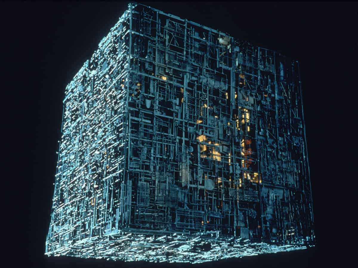
What’s the fastest speed we can see with the human eye? One way to answer this question has been suggested by Jack Singal, a physicist at the University of Richmond in Virginia. He imagined an object – a Borg spaceship from Star Trek if you like (shown above) – moving at speed v, passing linearly across one’s field of vision, visible if it were at rest, and directly overhead. For simplicity, he ignored any potential distortion from the atmosphere and assumed the ship is bright enough to see.
Now if A is the angle (in radians) over which the human eye can focus, T is the neurological “refresh rate” of human visual perception, and D is the closest distance between you and the object, then according to simple geometry, and ignoring any unfocused peripheral vision, v = DA/T. Given that A ≈ 1° (0.017 radians) and T ≈ 0.001 s, then if the Borg ship is 100 km away, skimming the very top of the Earth’s atmosphere, the fastest visible speed will be 1750 km/s or roughly 0.6% of the speed of light. (Such an object would take only four minutes to get from Earth to the Moon, and its purely relativistic length contraction would be, for a 1000 m-long ship, only 2 cm.)
However, that limiting observational speed may be too high. Jordan DeLong, a psychologist who is a data-science director of the Los Angeles market-research firm Research Narrative, thinks the situation is more complex. “The eye isn’t uniformly sensitive like a digital camera,” says DeLong, who has carried out research on vision especially as it relates to film. “The periphery is better at detecting motion, but not as sensitive to detail and colour.” And brighter visual stimuli are transmitted more quickly to the brain.
DeLong points to a classic study from 1985, in which a team led by Craig Meyer, now of the University of Virginia, immobilized the heads of five male subjects, who were asked to track a moving spot as closely as possible. Using a device to monitor their eye movements, Meyer found that – in this near-perfect set-up – their eyes could track a spot to an upper limit of about 90° per second (Vision Research25 561). “That could be a small object really close to the eye that’s moving slowly, or a large thing in the distance moving more quickly,” says DeLong. The equation above yields a maximum detectable velocity at a distance of 100 km of only about 160 km/s, or 0.05% of the speed of light.
Originally predicted at the end of the 1960s, researchers still can’t say with certainty that they have actually observed the supersolid phase of matter in the laboratory. Physicists in Austria now report that they have found further evidence for this phase in a Bose-Einstein condensate made of erbium atoms. The finding will help advance our understanding of how spontaneous symmetry breaking occurs in quantum systems, they say. It also confirms that ultracold atoms are a powerful test bed in which to study highly non-trivial quantum phenomena.
A supersolid is a paradoxical form of matter – it flows without friction (like a superfluid) but its particles are arranged in a crystalline lattice (like a solid). Indeed, it is described as being a state in which two continuous symmetries are broken at the same time. These are: the translational invariance, which is associated with crystalline order; and the gauge symmetry, which is associated with the material’s frictionless flow.
“The remarkable thing about a supersolid phase is that it has a dual nature in which two antithetic orders co-exist,” explains study team leader Francesca Ferlaino of the University of Innsbruck. “A supersolid is in fact both a crystal and a superfluid.”
Dipolar quantum gases could be supersolids
Researchers first predicted the existence of supersolidity in quantum solids with mobile bosonic vacancies. Later on, they focused on observing it in superfluid helium-4. Indeed, in 2004 physicists at Pennsylvania State University in the US reported on evidence for helium-4’s supersolidity, but further investigation by the team unfortunately revealed this not to be the case.
More recent experiments by three independent teams, including Ferlaino’s, have revealed that dipolar quantum gases elongated in one direction can undergo a phase transition from a regular Bose-Einstein condensate (BEC) to a state that has supersolid properties. The atoms in dipolar gases have large magnetic moments and it is the interactions between these atoms that give rise to supersolidity.
One team led by Tilman Pfau of the University of Stuttgart in Germany and the other led by Giovanni Modugno of the University of Florence in Italy found evidence of this solid phase in an ulracold gas of magnetic atoms (either erbium or dysprosium). “In this present work we have made an important step forward and have studied how this phase reacts to excitations, such as stretching and compression,” says Ferlaino.
In quantum physics, any system has distinct excitation modes that characterize how it responds to an external perturbation – similar to a bell that one strikes, she explains. “The bell responds with a given frequency that is associated with a given type of deformation. This can be a vibration, shear or compression of its constituents.
“We have now found that the solid phase in a cloud of ultracold erbium atoms responds to the excitations in a way that agrees with what is theoretically expected for a supersolid, thus providing further evidence for this state.”
Theoretical calculations and experiments
Thanks to a model-free statistical analysis known as Principal Component Analysis, the researchers were able to observe that the gas of supercooled erbium atoms develops two different energy states at the same time when it undergoes a phase transition from a BEC to a supersolid. This pair of states manifests itself as a distinctive structure in the energy-momentum spectrum of the system and forms two branches.
“Each of these branches is associated with one of the orders – crystalline or superfluid – and contains modes that are either vibrations of the crystal structure or superfluid respectively,” says co-team leader Lauriane Chomaz “In our work, we show both theoretically and experimentally that this crucial feature of the supersolid spectrum persists in laboratory systems of a finite size.”
The Innsbruck physicists then studied their system in an experiment by confining the erbium atoms into a 3D optical trap created by lasers (which is the usual way to create a BEC) that was elongated in one direction. To perturb the BEC and study its response, they quickly changed the size of the trap along this direction to expand and contract the condensate. The moving atoms interfere with one other and produce an interference pattern that contains multiple excitation modes belonging to the two branches – just as in the theoretical calculations.
Powerful test bed
These findings will help us better understand spontaneous symmetry breaking in quantum systems, Ferlaino tells Physics World. They also confirm that ultracold atoms are a very powerful test bed in which to confirm the existence of highly non-trivial quantum phenomena, and to simulate or control them.
The researchers, reporting their work in Physical Review Letters, say that they will now be characterizing the supersolid phase they have observed. “We will be particularly focusing on the superfluid flow in the system and how it evolves along the phase diagram,” says Ferlaino. “We would like to answer questions such as how does the system behave when it is rotated or locally perturbed? What other characteristics can we glean from the supersolid’s excitation spectrum – both in terms of its solid elasticity and its superfluid fraction?”
“I’d like to make people aware of the tremendous pressure we put on the most valuable ecosystems on Earth—in the tropics, for example—by shifting from a fossil-based to a bio-based economy without changing our consumption habits,” says Martin Bruckner of Vienna University of Economics and Business, Austria. “I am concerned that current environmental policies do no more than problem shifting.”
Seeking to promote “green growth” while reducing reliance on fossil fuels and petrochemicals, the EU’s Bioeconomy Strategy aims to increase the use of bio-based materials such as textile and oil crops. But while there are some environmental benefits to this approach, e.g. biofuels could help make transport less carbon-intensive, replacing resources with cultivated alternatives is not necessarily sustainable.
Bruckner and colleagues from Austria, Germany and Sweden combined two resource-use models to identify the origins and final destinations of a range of non-food agricultural products. The EU is both the largest consumer and net importer of embodied cropland, they found.
The results demonstrate a way to monitor the environmental effects of bioeconomic policies and could help the EU achieve its sustainable development goals.
Bruckner and colleagues set out to measure the EU’s non-food cropland footprint by tracking agricultural products from the field to the end consumer. They started with a biophysical model based on commodities and land-use data from the UN Food and Agriculture Organization. Although this model follows food products all the way to their final form, it accounts for non-food products only until they reach the industrial processing stage.
To complete the last part of the journey, the team correlated the output of the biophysical model with a database detailing the supply chains of hundreds of products across dozens of countries. In this way the researchers determined the cropland embodied in a range of agricultural commodities, and linked the country of consumption with the country of origin.
Although not the most intensive user of cropland per capita, in absolute terms the EU relies more on imported non-food biomass than any other region. Non-food products consumed in the EU embody nearly twice as much land as the EU uses for non-food agriculture within its borders.
Much of this biomass is imported from tropical countries—Indonesia in particular—where agricultural development comes at the cost of deforestation and biodiversity loss. Although such regions suffer the environmental damage of resource extraction, they do not necessarily gain the full benefit of the trade, as a large part of the value is added by industrial processing in the EU.
Quantifying the footprint of non-food agricultural products could lead to development strategies that share environmental harms and economic benefits more equitably between countries. It could also suggest opportunities to replace environmentally damaging products with more benign alternatives, but this alone will not be enough to mitigate the effects of the expanding non-food sector.
“Replacing palm oil with domestic rapeseed oil, for example, would require three times the land area,” says Bruckner. “Instead of problem shifting we need to focus on reducing consumption levels. This will be the only way we can really make a difference, reduce pressure on ecosystems, and mitigate biodiversity loss.”
The last full reversal of the Earth’s geomagnetic field took at least 22,000 years to complete, researchers from the US and Japan have revealed. The finding, which was derived by combining volcanic, sedimentary and ice-core records, suggests that reversals can take several times longer than was previously thought. It also further challenges the notion that a future reversal might be completed within a human lifetime.
The geomagnetic field is produced by the motion of the Earth’s liquid outer core, which acts as a dynamo. Although superficially stable – and presently reliable enough to navigate by – the field does change with time. At present, for example, the magnetic North Pole is in the process of drifting towards Siberia, while the field strength has been decreasing steadily by around 5% for each century since human records began.
Records in the rocks
With magnetically aligned minerals in certain rocks having left us with a record of the magnetic field at the time they were formed, we know that such a weakening can be a precursor to a so-called excursion – in which the magnetic poles shift by up to around 45 degree – or a full blown reversal, in which the field flips and settles upside down. These events, products of growing instabilities in the geodynamo, appear to occur every several hundred thousands years or so.
“Reversals are generated in the deeper parts of the Earth’s interior, but the effects manifest themselves all the way through the Earth,” explains Brad Singer, a geologist at the University of Wisconsin Madison.
Exactly what impact a future reversal might have on human civilization, navigation and communications, however, is unclear. And scientists still don’t understand what causes them, how long a reversal would take, and what the warning signs of one might be.
“Unless you have complete, accurate and high-resolution record of what a field reversal really is like at the surface of the Earth, it’s difficult to even discuss what the mechanics of generating a reversal are,” Singer notes.
Better measurements
To help develop a more accurate picture, Singer and his colleagues took magnetic readings of rock samples from seven lava flows from the Canary Islands, the Caribbean, Chile, Hawaii and Tahiti. They also determined the age of the samples using a newly-enhanced method of potassium-argon radioisotope dating.
“Lava flows are ideal recorders of the magnetic field. They have a lot of iron-bearing minerals and when they cool, they lock in the direction of the field,” says Singer. “But it’s a spotty record. No volcanoes are erupting continuously. So we’re relying on careful field work to identify the right records.”
The team complemented their lava-flow records with two other sources of data on the historic orientation of the geomagnetic field. The first of these were magnetic readings taken from the sea floor, which are less precise than those taken from lava flows – due to variations in sediment rates, weaker magnetization, and biological disruption that can smear the preserved magnetic orientations – but can provide a more continuous record.
Secondly, the researchers took measurements of beryllium deposits across time, as preserved in Antarctic ice cores. Beryllium is produced when cosmos rays hit the atmosphere, which means that periods in which the magnetic field was weaker – and therefore allows more radiation to pass through it – can be identified by increased beryllium in the ice cores.
Combined together, the various records allowed the researchers to piece together the nature of the geomagnetic field over a 70,000-year period centred around the Matuyama-Brunhes reversal – the last time the field completely flipped over, around 784,000 years ago.
Longer reversal
Singer and colleagues found that the final reversal was relatively rapid by geological standards, taking less than 4000 years. However, it was preceded by two individual excursions within a period of instability lasting 18,000 years – more than twice as long as recent research had suggested reversals should take.
“I’ve been working on this problem for 25 years,” said Singer. “And now we have a richer and better-dated record of this last reversal than ever before.”
Andrew Roberts, an earth scientist from the Australian National University who was not involved in the present study, said: “I take these results to indicate that the last magnetic polarity reversal occurred during a prolonged period of time in which Earth’s magnetic field was weak and unstable.”
Roberts also notes that it is still possible that the main reversal occurred rapidly. “There have been other prolonged unstable periods, such the Blake and post-Blake events between 120 and 90 thousand years ago, during which the field has been demonstrated to have changed extremely rapidly.”
Gillian Turner, a geophysicist from the Victoria University of Wellington who also was not involved in the study, agrees: “As the accuracy and resolution of dating both volcanic rocks and sedimentary sequences continues to improve, we should expect to see excursional activity associated with successful polarity reversals more and more often.”