Invented 50 years ago this month, atomic clocks have revolutionized how we measure time. But optical clocks, which use light rather than microwaves, promise to be even more accurate and could lead to the second being redefined

It is 50 years this month since Louis Essen demonstrated the first caesium atomic clock at the National Physical Laboratory and set in motion the shift to atomic timekeeping. Back then, the second was defined in terms of the period of the Earth’s rotation, but this was found to fluctuate as our ability to measure time improved. Essen showed that atoms, which have a set of discrete energy levels, could provide a much more stable reference time interval. In 1967, some 12 years later, the second was officially redefined by the Comité International des Poids et Mesures in terms of the gap between two specific energy levels in a caesium-133 atom.
Since Essen’s pioneering work, the accuracy of caesium clocks has steadily improved by a factor of 10 or so every decade, such that today’s best atomic clocks are accurate to better than one part in 1015. These improvements have led to many scientific advances as well as to technologies such as the Global Positioning System (GPS) and the Internet, which depend critically on time and frequency standards. Although this performance is impressive, a new type of device known as an “optical clock” could lead to even greater improvements.
In a standard atomic clock, a beam of caesium-133 atoms is probed by microwaves that have a frequency of about 9.2 x 10⁹ Hz. When the microwave frequency is adjusted to a value of exactly 9192 631 770 Hz, the photons have an energy that is equal to the energy difference between the two very closely spaced energy levels that make up the ground state of the caesium atoms. The atoms absorb the microwaves and a signal generated from the absorption is fed back to the microwave source, which stops it drifting from this specific frequency. The stability imposed on the microwave source by the atoms is what allows us to define the second as “the duration of 9192 631 770 periods of the radiation corresponding to the transition between the two hyperfine levels of the ground state of the caesium-133 atom”.

Optical clocks, in contrast, use light rather than microwaves. All other things being equal, the stability of an atomic clock is proportional to its operating frequency and inversely proportional to the width of the electronic transition. Since light has a frequency of about 1015 Hz – roughly 100,000 times higher than that of microwaves – clocks based on narrow transitions at optical, rather than microwave, frequencies should be much more stable. Clocks need to be both stable and accurate, with greater stability making it much easier and quicker to judge how accurate a clock really is. Optical clocks have many potential applications – from improved GPS measurements and better tracking of deep-space probes to fundamental tests of general relativity and measurements of the physical constants. They could even lead to the second being redefined once again.
Atomic clocks: from past to present
The use of atomic timekeeping has progressed steadily since Essen’s pioneering work (see box below). The clock that he developed 50 years ago at the National Physical Laboratory (NPL) was relatively primitive by today’s standards, having an accuracy of just one part in 1010. It used a beam of hot caesium atoms that had been evaporated from an oven. The atoms were probed using a technique that was originally developed by Norman Ramsey from Harvard University, for which he shared the 1989 Nobel Prize for Physics. It involved firing a short pulse of microwaves at one position along the beam, followed – a few milliseconds later – by another short pulse further along the beam. Interference between the excitation of the atoms by the two probe pulses creates a set of fringes as a function of the microwave frequency. These interference fringes, the widths of which are inversely proportional to the interval between pulses, sub-divide the absorption profile of a single pulse, thereby increasing the spectral resolution.

Various companies began to develop commercial caesium clocks based on Essen’s ideas, the best of which now have accuracies of a little better than one part in 1012. However, during the early 1990s a new type of caesium atomic clock known as an “atomic fountain” was developed by André Clairon, Christophe Salomon, Claude Cohen-Tannoudji and co-workers at the Observatoire de Paris and the Ecole Normale Supérieure. It was based on the pioneering work of Steven Chu and Bill Phillips, who in the mid-1980s developed techniques using lasers and magnetic fields to trap clouds of atoms that had been cooled to temperatures below 1 mK. In the fountain, cold caesium atoms are launched upwards to a height of about a metre before falling back under gravity. The atoms, which pass through a microwave cavity once on the way up and once on the way down, move so slowly that they interact with the microwaves for much longer periods than they would if they were hot.
This arrangement allowed Clairon to use time-separated “Ramsey pulses” to probe the atoms’ microwave absorption with a resolution of just 1 Hz – much less than the 100 Hz for the hot atoms in the caesium-beam clock. With such narrow features, fountain clocks are typically stable to about one part in 1015, provided that the fluctuations in the frequency of the clock are averaged over the course of a day. In other words, they can measure time to better than 100 picoseconds (10-10 s) per day.

Today’s best caesium-fountain clocks are now accurate to better than 1 part in 1015, and contribute as primary frequency standards to the international timescale. Indeed, atomic clocks are now so good that time and frequency can be measured more precisely than any other physical quantity. Not surprisingly, applications have blossomed. For example, atomic clocks can be found on board all 24 of the satellites that form the heart of the Global Positioning System. These clocks – together with ground-based clocks – enable sailors, pilots, drivers and walkers to know their location to within a few metres.
Enter the optical clock
Although caesium-fountain clocks are now very accurate, there are limits to how much better they could get. First, collisions between cold caesium atoms in the fountain can shift the frequency of the atomic transition. Second, the stabilities of one part in 1015 are only possible by averaging the signal over a period of about a day, which makes it hard to use the fountain clock at this level of accuracy in real time. Optical clocks, however, could meet our needs for better timekeeping. With frequencies approaching 1015 Hz – some 100,000 times higher than the 9.2 GHz microwave frequency of the fountain – optical clocks should be stable to almost one part in 1015 simply by averaging over just a few seconds, rather than a day. With longer averaging times, stabilities of one part in 1017 or better should be possible.
Optical clocks could have many applications. For example, while planes can navigate via GPS, it is not yet acceptable to land an aircraft by GPS alone because the atomic clocks on satellites are still not accurate enough and it takes too long to compute positions. Highly accurate clocks will also be useful for deep-space probes, which need to travel vast distances. Moreover, improvements in the ground-based “master clocks” that calibrate the GPS atomic clocks – along with better satellite clocks – will allow transportation systems to locate vehicles with sub-metre precision in real time. When integrated with mobile-phone technology, the commercial possibilities of such developments are immense.

Highly accurate clocks could also help us to measure fundamental constants and test the laws of physics, such as Einstein’s theories of special and general relativity. Some theorists believe that the fine-structure constant, α, which characterizes the strength of the electromagnetic interaction, may have changed over the history of our universe (see “Are the laws of nature changing with time?” Physics World April 2003 pp33-38). If confirmed, the results would be of huge significance in cosmology and for theories that attempt to unify the four fundamental forces of nature.
One of the best ways of searching for present-day variations of a is to compare the frequencies of different types of atomic clock over the course of several years. While this is a short period of time compared with cosmological timescales, this approach can provide results that are competitive with rival astrophysical measurements due to the high frequency resolution achievable. The better the clocks, the smaller the variations in α that could be detected, with the current limit approaching one part in 1015 per year.
Inside an optical clock
There are three main elements to an optical clock. The first is a highly stable reference frequency provided by a narrow optical absorption in an atom or ion. This “clock transition” will typically have a natural line width of a few hertz or less. The second element of the clock is a laser, known as a “local oscillator”, which should also have a very narrow line width so that it does not broaden the atomic transition. The third component is some way of counting the extremely rapid oscillations of the local oscillator; these oscillations are the “ticks” of the clock. A device called a femtosecond comb is used for this part of the device (see “femtosecond comb”).

Critical to the performance of an optical clock is the first element – the clock transition. This needs to be as narrow as possible to make the clock stable. Its frequency should also be unaffected by external perturbations such as electric and magnetic fields so that the clock is as accurate as possible. The ideal frequency reference would be a single, motionless atom, unperturbed by any interactions with other atoms or the environment. We can come fairly close to this utopia by trapping a single ion in the tiny gap between the electrodes of an electromagnetic trap (figure 1). This trapping allows the ion to be laser-cooled to a temperature of about 1 mK and be confined to a region of space just a few tens of nanometres across. The clock transition is therefore not broadened by the effects of temperature or motion.
To probe the clock transition one needs a highly monochromatic laser, which can be achieved by stabilizing the laser frequency to a mode of an environmentally isolated low-drift optical reference cavity. Lasers with line widths that are less than 1 Hz have been achieved with this approach by groups at the National Institute of Standards and Technology (NIST) in Boulder, Colorado, the JILA lab at the University of Colorado and NPL.
Unfortunately, it is not easy to monitor the light being absorbed because narrow transitions are intrinsically very weak. The solution lies with a technique developed by the Nobel laureate Hans Dehmelt, which enables the absorption to be detected with almost 100% efficiency. Known as “electron shelving”, the technique is based on the fact that when the ion absorbs the probe light, it jumps to a long-lived excited state, where it remains for about a second. During this time, the ion cannot be laser-cooled – the process where the ion repeatedly jumps between its ground state and a short-lived excited state, absorbing and re-emitting photons at the cooling wavelength.
The upshot is that when the ion is “shelved” in the long-lived excited state, no fluorescence photons from the cooling transition are emitted. The absence or presence of this fluorescence tells us whether the probe light has driven the ion to the long-lived state or not (figure 2). By measuring the probability of the ion jumping to the long-lived state as a function of the frequency of the probe laser, we can observe the narrow spectral profile of the clock transition. The frequency of the laser light can then be stabilized to the centre of this profile, where the transition probability is at a maximum.
A number of labs around the world are investigating optical clocks using various species of ion. The choice of ion depends on several factors, such as how narrow the clock transition is, the wavelengths of the lasers that are needed to cool and probe the trapped ion, and the predicted sensitivity to external perturbations, which can shift the transition frequencies.
In 2000 Jim Bergquist and co-workers at NIST observed a cold-ion clock-transition line width of just 7 Hz at 282 nm in a single mercury-199 ion – the narrowest of any such clock transition to date. This is only a factor of four greater than the intrinsic natural line width of 1.7 Hz. Meanwhile, researchers at the Physikalisch-Technische Bundesanstalt (PTB) in Braunschweig, Germany, are studying a clock based on the 435 nm transition in ytterbium-171 ions, while groups at NPL and the Canadian National Research Council are investigating clocks based on the 674 nm transition in strontium-88 ions. All these experiments currently demonstrate line widths within a factor of 10 of the mercury line width.
Researchers in all of these groups have already stabilized the clock-laser frequency to the centre frequency of these narrow clock-transition profiles. In this way, frequency stabilities of better than one part in 1015 have been demonstrated for the mercury-199 clock and the ytterbium-171 clock when averaged for about 100 s and 1000 s, respectively. Ensuring that these clocks are affected as little as possible by external perturbations will be a key challenge.
Other ions being studied include some where the upper state of the clock transition is extremely long-lived, thereby allowing full benefit to be gained from the narrowest 0.1 Hz probe-laser line widths available. For example, researchers at NIST are studying a clock based on an aluminium-27 ion in which the upper state lasts for 30 s, while scientists at NPL are experimenting with a clock based on an ytterbium-171 ion in which the upper state lasts for an incredible six years! The only snag with the NIST clock is that the aluminium ion would have to be cooled using an extreme-ultraviolet laser, which is a formidable challenge.
Instead, Dave Wineland, Bergquist and co-workers at NIST are using an interesting experimental arrangement whereby the aluminium-27 ion is trapped with another species of ion – beryllium-9 – that can be cooled more easily. Laser-cooling the beryllium ion “sympathetically” cools the aluminium ion. The researchers cannot, however, probe the weak aluminium clock transition using the electron-shelving technique because there is no strong cooling fluorescence from the aluminium ion. Instead, Wineland and colleagues call upon techniques they developed for quantum-information-processing experiments, which enable information about the clock profile to be “mapped back” to the beryllium ion for read-out.
Clocks from clouds of atoms
Although single trapped ions could lead to highly accurate atomic clocks, they are not perfect. In particular, the signal-to-noise ratio of the atomic absorption signal – and thus the stability of the clock – is compromised because there is only one ion in the trap. One possible alternative is to use weak transitions in clouds of a million or so cold atoms. Clocks that use such transitions should be very stable because the stability is directly proportional to the square root of the number of atoms contributing to the signal.
The bulk of the work in this area has been carried out at the PTB and at NIST. Researchers there have focused on neutral calcium atoms, which have a weak transition at 657 nm with a natural line width of about 400 Hz between the 1S0 ground state and the 3P1 metastable state. In these experiments, the calcium atoms are laser-cooled to a few millikelvin in a “magneto-optical trap” similar to that used for cooling caesium atoms before they are launched in a caesium fountain. The problem is that the cooling light strongly perturbs the atoms, which means that it has to be turned off before the 657 nm clock transition can be probed. As a result, the atom cloud expands under gravity during the probe pulse and so has to be recaptured and recooled before it can be probed again. The rapid expansion means that the atoms can only be probed for a very short period of time, significantly broadening the atomic transition. Nevertheless, various tricks – including extra cooling of the atoms to 12 μK and applying two probe pulses about a millisecond apart – have led to accuracies of one part in 1014.
So how can these atomic optical clocks be improved? One option is to use a narrower clock transition, such as the 698 nm 1S0–3P0 transition in neutral strontium, which offers a line width of just 10-3 Hz. However, to use these narrower clock transitions you need a way of lengthening the interrogation time. One solution was presented in 2001 by Hidetoshi Katori from the University of Tokyo, who suggested confining the cooled atoms in what is known as an optical lattice.
An optical lattice is a region of space where standing light waves overlap to create a 3D potential that rises and falls periodically with position. The lattice has regular sites that are less than a wavelength apart, in which atoms can be trapped – a bit like eggs in an egg box (figure 3). By holding the atoms in the lattice sites, Katori reasoned, they could be probed for as long as one likes. One possible pitfall is that the trapping light beams will perturb the atoms and change the frequency of the clock transition. However, Katori proposed that the optical trap should be created with light at a “magic” wavelength of about 800 nm, where the shifts of the upper and lower levels of the strontium clock transition are exactly equal. The transition frequency will therefore be insensitive to intensity.
A number of groups are working on this lattice idea using strontium and ytterbium. The combination of high stability and low systematic frequency shifts provided by these atoms may offer the best of both worlds in the future.
Counting optical frequencies
One of the key challenges in building an optical clock is to count the “ticks” – the oscillation of the light source. However, light oscillates so fast – roughly once every femtosecond (10-15 s) – that it would be impossible to count individual oscillations using any conventional electronic device. The solution is to use a device called a “femtosecond comb”. First demonstrated in 1999 by Ted Hänsch and his group at the Max Planck Institute for Quantum Optics in Garching, Germany, this device bridges the gap between the microwave and optical regions of the spectrum in a single step.
The comb consists of a “mode-locked” femtosecond laser, which emits a train of pulses at a typical repetition rate, frep, of a few hundred megahertz. In the frequency domain, the sequence of pulses appears as a series of equally spaced frequencies – rather like the teeth of a comb. The frequency of any line in the comb is an integer multiple of the comb spacing (nfrep) plus an offset frequency (f0), which depends on the difference in the group velocity and phase velocity within the laser cavity. The all-important tick rate, fopt, is related to frep and f0, both of which can be determined experimentally.
The comb spacing, or repetition rate frep, can be measured from the beat signal between adjacent comb modes (figure 4). The simplest way of determining f0 is to have a comb that spans a complete optical octave, i.e. a factor of two in frequency. Some femtosecond lasers can now produce an octave-spanning comb directly. Alternatively, a short piece of microstructured fibre, in which an array of air holes surrounds the fibre core, can be used to broaden the spectrum by means of nonlinear frequency-mixing effects in the fibre.
With frep and f0 stabilized to a microwave atomic clock – and thereby compared with the caesium primary frequency standard – the comb can be used to measure the frequency of an optical standard fopt. This is done by determining the beat frequency between the optical frequency and the precisely known frequency of the nearest comb mode. However, as first demonstrated in 2001 by Scott Diddams and colleagues at NIST, it is also possible to turn this process on its head and to stabilize the comb to an optical standard rather than to a microwave standard. The comb then acts as the “clockwork” of the optical clock, dividing the optical frequency to produce a countable microwave output frequency frep.
Future times
Several groups have shown that femtosecond optical-frequency combs are a reliable way of comparing optical frequencies at the level of one part in 1019. As a result of comb developments, the accuracy of optical-frequency measurements has risen dramatically over the past few years, and is fast approaching the limit set by the current, caesium-based definition of the second (figure 5). The best published measurement of an optical frequency is that of the strontium-ion standard at NPL, which has an uncertainty of 3.4 parts in 1015 (see Margolis et al. in further reading). However, researchers at NIST have just reported a preliminary measurement of the mercury-ion standard with an uncertainty of 1.5 parts in 1015, which is very close to the uncertainty of the caesium standard.
If optical-frequency standards become more reproducible than caesium-fountain standards, a primary standard for time that is based on an optical clock could be on the cards within a decade or so. But given the many different species of atom or ion that are currently being investigated, much research is still needed to work out which is the best. Whether or not a clear front runner emerges, two things are highly likely. First, the powerful femtosecond-comb techniques will play a key role in comparing the accuracy of different clocks. Second, reproducibilities of one part in 1017 or 1018 will be reached.
To do any better, we will have to work even harder at stabilizing environmental factors such as magnetic and electric fields. The effects of general relativity will also become highly significant; after all, two clocks that are separated by just 1 cm in height will have transition frequencies that are gravitationally redshifted by one part in 1018 with respect to each other. Experiments comparing optical clocks in remote locations will therefore become a major challenge. Despite these difficulties, optical clocks are here to stay and will have applications – ranging from communication and navigation to fundamental physics – of which Louis Essen, half a century ago, could never have dreamed.
Defining moments in atomic timekeeping
1949 Ramsey’s separated oscillatory field technique
1955 First caesium atomic clock
1960 Hydrogen maser
1967 Redefinition of the second in terms of caesium
1975 Proposals for laser cooling of atoms and ions
1978 Laser cooling of trapped ions
1980s GPS satellite navigation introduced
1985 Laser cooling of atoms
1993 First caesium-fountain clock
1999 First optical-frequency measurement with femtosecond combs
2001 Concept of an optical clock demonstrated