Accurate measurement of temperature is a key part of almost every science experiment, and in most cases, the measurement is relatively straightforward. However, with my colleagues Robin Underwood and Gavin Sutton at the National Physical Laboratory (NPL) in the UK, I have just spent six years measuring a single temperature – and we knew the answer before we started! Sort of.

Every measurement is a comparison of an unknown amount of a quantity with a standard amount of that quantity. But in most measurements this “comparison against a standard” is indirect and not immediately apparent to the user. For example, when a shopkeeper weighs out 500 g of grapes, neither they nor their customer are immediately aware of the calibration chain that stretches from the shop, via the local “weights and measures” laboratory, to NPL and on to the unique lump of metal in the vaults of the International Bureau of Weights and Measures (BIPM) in Paris that is our standard kilogram.

For temperature, the standard amount to which all other temperatures are compared is the temperature of the triple point of water, T_TPW. To be sure, most people using a thermocouple to measure the temperature of an oven are not aware of this, but it is still true. If you were to visit NPL you would find a dewar filled with glass cells containing water held at its triple point, the temperature of which we use to directly calibrate thermometer readings.

At T_TPW, liquid water, solid ice and water vapour co-exist in equilibrium and this is chosen as the standard temperature because it can be reproduced relatively easily with an uncertainty below 0.001 °C. Currently, T_TPW is defined to be 273.16 K (or 0.01 °C) exactly. Scientists could have chosen any number to associate with this temperature, but this particular choice is made so that the magnitude of both a kelvin and a degree Celsius is close to the historical degree centigrade.

This definition has served us well for more than 50 years. But for many scientists – myself included – it is unsatisfactory. The reason that temperature is defined this way is a hangover from the fact that we learned to measure temperature before we understood what temperature was. If, 200 years ago, we had understood that temperature was a measure of the energy of atomic motion, we would have defined temperature directly in terms of energy. And that is what we now hope to do.

In statistical mechanics, temperature always occurs in combination with the Boltzmann constant, k_B. Currently, because T_TPW is defined exactly, if one measures the product k_BT_TPW then all the uncertainty in the product is expressed as an uncertainty in k_B. We think this is irrational and that k_B should be – as its name implies – a constant, and defined exactly.

In this conception the kelvin would be defined by k_B, which – like the speed of light in vacuum – would have an exact value with no associated measurement uncertainty. Since the units of k_B are joules per kelvin, this will relate temperature directly to energy, and link it firmly into the rest of the International System of Units (SI). In that way, in future, every temperature measurement will be fundamentally a measurement of the energy of atoms and molecules.

Our work is part of a wider effort to redefine the base units of the SI in terms of natural constants. The second and the metre are already defined in this way, and metrologists are busy worldwide trying to achieve the same goal for the kilogram, ampere and mole, an effort discussed in depth in Robert P Crease’s March 2011 article “Metrology in the balance”.

A sound approach

Our approach to measuring k_BT_TPW was to make life easy for ourselves and pick a physical system in which we could achieve the lowest possible uncertainty. Back in 2007 we thought hard about all the possibilities and chose to make a measurement of the speed of sound in a monatomic gas. There were two compelling reasons for this choice.

In future, every temperature measurement will be fundamentally a measurement of energy

First, the speed of sound in the limit of low pressure, c₀, in a monatomic gas is directly related to the root-mean-square speed of molecules, v_RMS, by the strikingly simple relationship c₀ = √(5/9)v_RMS. So if we could measure c₀with low uncertainty, then, if we knew the mass of the molecules, m, we could directly estimate the average kinetic energy of molecules, ½mv²_RMS. Statistical mechanics tells us that for a lowdensity molecular gas this is equal to 3 × ½k_BT. For more detail on the equations, see “Pinning down the product”.

The other reason for choosing to measure the speed of sound in a monatomic gas is that it is possible to make amazingly precise measurements of this value. The most obvious method for doing so is to measure the time it takes for a sound wave to travel a fixed distance. The measurement becomes more accurate as one makes the distance longer but that makes knowing the temperature over the whole path very difficult. The “trick” is to use a resonator.

In this technique one “folds back” the sound path so that it bounces around inside a cavity. Normally the sound from each reflection interferes destructively with sound from the loudspeaker and the sound pressure level inside the resonator is low. However, if one picks a frequency at which multiples of the wavelength precisely match the dimensions of the resonator, then constructive interference – resonance – takes place. By measuring the frequencies at which this happens it is possible to deduce the speed of sound, knowing the dimensions of the resonator.

One of the main advantages of this technique is that the speed of sound can be found independently from several different resonances varying in frequency from about 2 to 20 kHz. So the extent to which they agree provides a powerful self-checking feature. The problem is that although frequencies can be measured very accurately, it is much more difficult to measure the dimensions of the resonator. And even more challenging, the dimensions will of course change with temperature and pressure. We therefore had to choose the shape of the resonator very carefully.

In our work at NPL, we have been using a resonator in the shape of a triaxial ellipsoid. It is almost perfectly spherical, except that its x-, y– and z-radii, each approximately 62 mm, differ from each other by ±0.05% (32 µm). It might seem strange that distorting a sphere could result in a better measurement, but it does. The reason is that we used microwave resonances to measure the resonator’s internal dimensions and – unlike acoustic resonances – microwave resonances are degenerate in a sphere. This does not mean that the resonances are lacking in moral character; it means instead that there are several resonances with the same frequency. The triaxial distortion we created “lifts” this degeneracy, allowing us to measure a single resonant frequency for each principal radius. Our ability to measure the x-, y– and z-radii with nanometre resolution at the same time as measuring the acoustic resonances means any thermal expansion of the resonator can be accounted for.

Finally, we cooled the experiment to T_TPW. We knew the temperature was correct because we had previously calibrated six resistance thermometers in a cell containing water, ice and water vapour in equilibrium. We transferred these thermometers into our apparatus without disconnecting even a single wire in case this caused a spurious change in voltage that might be mistaken for a temperature change.

So our experiment worked like this. By measuring microwave resonant frequencies, we could estimate the size and shape of the resonator. Then, knowing the size and shape of the resonator, measurements of acoustic resonant frequencies allowed us to infer the speed of sound. We measured the speed of sound of seven resonances at different pressures and extrapolated to the limit of zero pressure (figure 1). This told us the limiting low-pressure speed of sound, c₀, and from this we could infer the mean molecular speed and hence the mean molecular kinetic energy, and hence k_BT. And finally, because we carried out the experiment at T_TPW, which is currently defined exactly, we were able to deduce k_B with low uncertainty.

This type of experiment – the results of which may affect the future assigned value of the Boltzmann constant – requires a very defensive approach. So we do not claim to have the right answer. What we are claiming is that we can prove that the right answer – whatever it is – cannot differ from our answer by more than our specified uncertainty. To make this claim stack up, we need to separate the final result into a number of sub-results and evaluate each of those in different ways and see if the answer changes. In this experiment there were three quite distinct parts: a measurement of how close we were to T_TPW; a measurement of the molar mass of the argon we used; and a measurement of the speed of sound, which depended critically on the size and shape of the resonator.

Sadly, the features editor of Physics World flatly refuses to turn over this entire section of the magazine to a discussion of our experiment, so here are two highlights of the measurement, concerning our estimate of the radius of our resonator and our estimate of the speed of sound.

Precision engineering

In order to reach our target of measuring k_B with an uncertainty below one part in 10⁶, we needed to measure the average, a, of the resonator’s three radii with an uncertainty substantially less than 0.5 parts in 10⁶, or roughly 31 nm, on a radius of 62 mm. This was – to put it mildly – challenging. So we chose to begin by making the resonator from two hemispheres, each manufactured with breathtaking precision.

For this we enlisted the help of Paul Morantz and colleagues at Cranfield University in the UK, who are more used to sculpting mirrors for space telescopes. It took months to design the apparatus to simply hold the hemisphere on the lathe without straining the copper. Long experience had taught Morantz that to create two perfect quasi-spheres, we would need to start with eight “blank” hemispheres, and pick only the best candidates to make the final cut that defines the inner shape.

A triaxial ellipsoid has no rotational symmetry, and so to create such a shape on a lathe is a challenge. The angular rotation of a hemisphere must be measured in real time, and the single-crystal diamond-cutting tool moved back and forth in synch with the rotation (figure 2a). This involved adjusting the position and speed of the tool thousands of times a second by a program written in MATLAB. Morantz considered every aspect of the interaction of the diamond tool as it cleaved through the copper, and specified where the tool should be at every millisecond. The result of all this effort is an artefact of stunning beauty with a mirror finish with only nanometres of surface roughness.

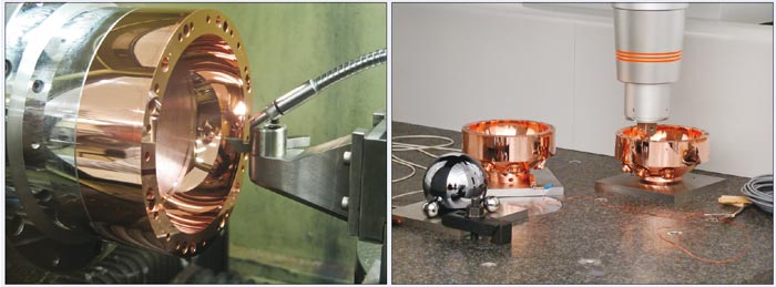
The resulting four hemispheres were measured using a mapping instrument known as a co-ordinate measuring machine (CMM), and shown to be within 1.5 µm of their design shape over the entire surface. At the same time as we measured the hemispheres, we also made measurements on a highly perfect silicon sphere the size of which we already knew (figure 2b). In this way we could correct for errors in the CMM and we eventually achieved an uncertainty of measurement of 132 nm on the average radius. Not bad, but not good enough.

One difficulty was that to estimate the shape and size of the resonator when assembled, we had to take account of the fact that the flat surfaces of the hemispheres were only flat to within a wavelength of light – and so they did not quite mate perfectly. We also had to consider the changing shape of the hemispheres as we tightened the bolts to hold the hemispheres together.

To measure the average radius of two assembled hemispheres we used microwave resonances. This involved inserting two tiny wire antennas so that they were just flush with the inner surface. When the wavelengths of microwaves just fit inside the resonator, the transmission from one antenna to the other increases strongly. By measuring the frequencies at which these resonances occurred we could estimate the average radius in terms of the speed of light.

Crucially we did this with eight different resonances at frequencies from 2 to 20 GHz and the results agreed within a staggeringly tiny uncertainty of just ±3.5 nm. When one encounters this level of consistency in an experiment one has to concede that nature is trying to convey a message. Inserting acoustic transducers into the sphere – so we could measure the speed of sound – made the agreement between radius estimates from different microwave modes a little worse but our final uncertainty estimate was still only 11.7 nm. Which was good enough for us.

So because of all these checks, we feel confident in our estimate of the average radius because although we have tried, we cannot see any way that it could be wrong by more than about 11.7 nm.

Skinny sound peaks

The propagation of sound through a gas consists of a repeating cycle of exchange between thermal and mechanical energy. As the gas is compressed it becomes heated, and energy is stored as compression of the gas. As it expands, it cools and the thermal energy is transformed back to mechanical energy.

In the bulk of the gas this process is almost lossless, but for our estimate of the speed of sound we had to consider that within approximately 0.01 mm of a solid wall, the heat of compression is quickly “wicked” away, resulting in loss of energy in a so-called thermal boundary layer.

It took months to design the apparatus to simply hold the hemisphere on the lathe

For a monatomic gas, the speed of sound should not depend on frequency in the acoustic range. So using a resonator we were able to check our answer by working out the speed of sound from several different resonances over a wide range of frequencies. For each resonance the effect of the thermal boundary layer is different and so we had to apply an adjustment based on our theoretical understanding of the thermal boundary layer. Adjusting data makes us uncomfortable, but we are confident that we have done this correctly because estimates of c₀ based on different resonances agreed with an uncertainty of only 0.09 parts in a million.

However, when we looked at the widths of our resonances, we were not pleased: we found that they were narrower than expected. In one extreme case a resonance with a frequency of 3548.8095 Hz was expected to be 2.864 Hz wide, but instead we found the width to be 2.858 Hz. We were flummoxed.

When energy is lost as sound bounces around inside the resonator, the frequency profile of each resonance broadens. So having resonances that are too broad is understandable – it means there is a little bit of extra loss somewhere in the resonator. But having resonances that are too narrow meant there was something going on in the resonator that we did not understand. And since we were unaware of what this thing was, we could not easily assess how wrong it could make our answer.

However, after publishing the “line-narrowed” data at the 9th International Temperature Symposium in 2012, a colleague from the National Institute of Standards and Technology in the US, Keith Gillis, showed us the results of his new theory of a spherical resonator on which he had been working. His theory evaluates the effect of the thermal boundary layer to an additional level of precision. To our surprise and relief, his theory matched closely what we had observed. It was not that our resonances were too narrow, it was the theory that had not been sufficiently developed.

Making it official

In July Metrologia published our new estimate: k_B= 1.380 651 56 (98) × 10^–23 J K^–1 where the (98) represents the uncertainty in the last two digits (Metrologia 50 354). The relative standard uncertainty is 0.71 × 10^–6 , significantly less than our target of 1 × 10^–6 , so personally, my work is done.

But NPL has not been working alone. Through 2014 we expect further estimates to be submitted to the Committee on Data for Science and Technology, which will consider their uncertainty estimates and relative consistency and come up with a recommended value and an uncertainty.

And then if the various committees and sub-committees of the BIPM agree, a proposal will be made by the International Committee on Weights and Measures to change the definition of the kelvin. If that is agreed by the General Conference on Weights and Measures when it meets in either 2014 or 2018, then the relative standard uncertainty of k_B and T_TPW will swap places: the value of k_B will become exact and the value of T_TPW will become uncertain. If the eventual uncertainty is close to 0.7 parts in 10, then the uncertainty in T_TPW would become 0.19 mK.

You may at this point be wondering whether you will be affected by this change. Let me reassure you: you will not. I can be confident of this because almost everyone in the world measures temperature according to a procedure called the International Temperature Scale of 1990, which specifies how to practically calibrate thermometers, and for the moment, nothing in this procedure will change.

However, since 1990 we have discovered that temperatures estimated by this procedure (called T₉₀) are slightly in error in that they differ from thermodynamic temperature – the familiar T in your equations of physics. The extent of this error is small by most people’s standards, with T–T₉₀ growing from zero close to T_TPW to about +4.5 mK at 29 °C and, –9 mK at –100 °C.

So having spent six years making the one temperature we thought we knew a little more uncertain, we have now begun using our resonator – currently the most accurate thermometer in the world – to measure T–T₉₀. And hopefully that will eventually make everyone’s temperature measurements a little more certain.

Pinning down the product

In our experiment to redefine the kelvin in terms of natural constants, we sought to measure the Boltzmann constant, k_B, via its product with T_TPW, the temperature of the triple point of water; the product k_BT_TPW is related to the average kinetic energy of a gas molecule.

We first worked out the speed of sound, c, in a resonator of average radius a from the resonant frequencies, f_n, using c = 2πaf_n/Z_n, where Z_n are characteristic numbers for each resonance (called eigenvalues).

We extrapolated several measurements of the speed of sound to find its limit at low pressure, c₀, then worked out the product k_BT_TPW using 3/2 k_BT_TPW = 1/2 mv²_RMS = 1/2 m [9/5 c²₀], which simplifies to k_B = 3mc²₀/5T_TPW

So by getting close to T_TPW, and measuring c²₀ and the average mass of the gas molecules, we could make an estimate for k_B. Since the units of k_B are joules per kelvin, or m² kg s^–2 K^–1 , the value of k_B links the kelvin directly to SI base units.