Activists protesting against genetically modified organisms recently destroyed a field trial of genetically modified rice in the Philippines. Participants and sympathizers claimed that the crop was poisonous, would destroy biodiversity and was a means for industry to exploit the poor.
But the rice had no known health hazards. It did not dominate other rice species and thus would not threaten biodiversity. It had been altered to create beta carotene – a precursor to vitamin A, which counteracts blindness and other illnesses associated with weakened immune systems, thereby helping hundreds of thousands of children lacking vitamin A. The rice was developed not by industry but the International Rice Research Institute, a non-profit organization.
The Philippine vandalism, however, harmed far more than the rice and its intended beneficiaries. It damaged the credibility of the entire scientific infrastructure that created the rice and determined it to be safe.
This controversy is but one of several instances – including fracking, nuclear power, climate change, vaccination and evolution – playing out in ways that marginalize expertise and make scientific evidence seem irrelevant. One may have sound non-scientific reasons for opposing things like genetic modification, such as not wanting to “instrumentalize” nature. But making good judgments requires respecting what science has discovered about the world and debating issues on their merits. Marginalizing science allows such controversies to unfold as “morality plays” about social inequalities or injustices, or only about politics or economics, rather than as complex negotiations between what we want and what is possible. Inevitably, bad decisions result.
Never in history have good judgments about issues such as energy, pollution and health depended more on science. Yet incorporating science into such debates has been beset by saboteurs, undermined by politicians and met with scepticism. Why?
Three reasons
The answer lies in three separate entangled ingredients, which I dub “manipulated acoustics”, “impure science” and “magical thinking”.
“Acoustics” refers to the way partisans of positions are ever more adept at mimicking and manipulating the voice of science itself. They do this by manufacturing facts and spreading pseudo-evidence, generating pseudo “experts”, using celebrities as spokespeople and taking advantage of the media’s penchant for granting equal time to different sides of an argument, and priority to what’s extreme and photogenic. I needn’t supply examples; you can find them yourself. These factors amplify voices in a controversy regardless of their integrity.
By “impure science”, I mean the way partisans often denounce scientific findings they don’t like. They point to discrepancies between how these findings were produced and the image of science we learned in school as emerging “from nowhere”: pure, value-free and definitive. If a particular study was partly funded by a pharmaceutical company, if a model depends on projections rather than certainties, or if someone has ties to the nuclear industry, the results must be suspect, they claim.
Just saying no Anti-fracking protest in Balcombe, UK, in August 2013. (Courtesy: iStockphoto/rsokoloff)
Finally, and surprisingly, scientific advance itself implicitly promotes a harmful “magical thinking”. This curious phenomenon was first identified by the Italian philosopher Giambattista Vico almost 300 years ago in his 1725 book New Science. Vico pointed out that the very maturation of human thought tends to foster an over-reliance on analytical rationality that encourages people to indulge themselves and view the world’s resources as at their disposal. The very success of science and technology, in other words, encourages the illusion that almost everything is within our grasp.
This magical thinking makes us feel like free agents – entitled to choose our forms of energy, nutrition and environmental conditions, without having to make severe, costly and risky trade-offs. It’s an illusion that’s amplified by powerful money and political influence. Don’t like fossil fuels but scared by nuclear? Go solar! Hate starvation but creeped out by genetic manipulation? Grow more food! And if we can’t do these things, it must be someone else’s fault, probably a conspiracy. We are accustomed to relying on our benefits but resent having to pay for the infrastructure that produced them. As one US congressman remarked – my informant heard it first-hand but insists on remaining anonymous – “Why do we need Landsat satellites when we have Google Earth?”
The critical point
How, then, can we deal with these problems?
Contending with wonky acoustics requires patiently tracking down and exposing fabrications and misrepresentations – a task for scientists and the sceptics movement. It is tedious and time-consuming for sure, but there is a silver lining: when partisans manipulate acoustics they at least presuppose that offering evidence and appealing to experts is how such debates should work.
Dealing with charges of impure science, meanwhile, is not a task for scientists but science educators. Science education needs to convey the reality that real science does not emerge “from nowhere” but from real people with passion, values and commitments. Science, we need to remind everyone, is our best tool for navigating the complex modern world filled with a fear of hazards and people who manipulate and prey on that fear.
As for countering science-induced magical thinking, that is not a task for either scientists or educators but for the humanities. It would require an improved human self-recognition; making better known the full story of how human thought and institutions evolved, and how some things are gained and others lost with each step. Realizing progressive human ambitions, we need to remind ourselves, usually comes with hidden costs.
There is, in short, no quick fix for repairing the dismal way we resolve controversies. It won’t work simply by restating the importance of science, which would only make science appear like one lobby among others. Vico thought the solution required the development of what he called a “new science”; today, it will require revamping science, science education and the humanities for the 21st century.
A new method for imaging the flow of blood has been developed by researchers in the US. By using ultrasound to thermally tag blood, along with photoacoustics to image the resulting heat flow, the new technique is considerably more sensitive than the conventional Doppler ultrasound method that is currently used. While presently at the in vitro testing stage, this technique might have a variety of clinical applications, especially in medical diagnosis.
Being able to image the flow of blood within deep tissue would provide valuable information for the diagnosis and understanding of many diseases, with potential applications including functional brain imaging, detection of vascular diseases (such as atherosclerosis – the thickening of artery walls with calcium and fat) and the analysis of blood within tumour microenvironments (commonly having complicated vasculatures with intermittent blood flows), which could help in the early detection of cancer.
Going with the slow flow
Currently, flow imaging is undertaken through Doppler ultrasound (or sonography) in which the flowing blood causes a Doppler shift in the reflected ultrasound waves that can be measured and used to discern the flow rate. However, this technique has its limitations. Doppler ultrasound has poor sensitivity to blood, which weakly scatters in comparison with tissue. This issue is even more pronounced at the low frequencies that are commonly used to probe deeper into flesh. At slow flow rates, the small Doppler shifts from the moving blood can therefore be difficult to distinguish from shifts that are caused by the surrounding tissues. Indeed, the effect is undetectable for blood flowing slower than about 10 mm s–1.
One possible alternative to Doppler ultrasound is photoacoustic imaging, which uses short pulses of low-energy laser light to locally heat the target for analysis. This heating results in thermal expansion, creating ultrasound waves in proportion to the optical absorption of the target tissue. When recorded, this emitted ultrasound can therefore be used to create a map of the target’s absorptivity. While this method works well at shallow tissue depths (up to 1 mm deep), flow sensing in deep tissue is hindered by the high densities of blood cells.
Thermal tagging
Photoacoustic imaging is, however, very sensitive to temperature variations. Taking advantage of this, Lidai Wang and colleagues at the Washington University in St Louis have developed an alternative method of analysing blood flow by combining photoacoustic imaging with thermal ultrasound tagging that they refer to as “photoacoustic flowgraphy”. The researchers used focused ultrasound to locally heat a fixed part of a blood vessel and mapped out the resulting temperature distribution along the vessel as the blood flowed downstream.
As the laser pulse expands the material, it generates sound waves of a particular amplitude that, in turn, vary with the temperature. In a test set-up, the team could see how the heated sample moved by tagging the sample with the laser 10 times a second. Comparing subsequent images of the sound waves (taken using an array of detectors) allowed the researchers to follow the flow in a 1.5-mm tube of cow’s blood, including its faster speed at the centre of the tube.
“The spatial frequency (or period) of the temperature distribution changes with blood-flow speed,” explains Wang, with blood that flows faster generating a longer spatial period and a lower spatial frequency. This enables the flow speed to be calculated from the spatial frequency of the photoacoustic images recorded. Compared with traditional Doppler sonography, photoacoustic flowgraphy is considerably more sensitive, enabling the team to measure capillary-level blood flow at speeds as low as 0.24 mm s–1. “[This] is four times slower than Doppler sonography,” Wang adds. Furthermore, use of spectral photoacoustic imaging with this new method could provide other useful functional information, such as the blood’s oxygen saturation and even the metabolic rate of oxygen.
Assessment tool
“What I find particularly exciting is how this can be combined with functional and anatomical photoacoustic imaging to determine several tumour properties at once using one measurement,” comments Eric Strohm, a biophysicist at Ryerson University in Canada who was not involved in this study. “While in the early stages of development, this technology could eventually see clinical applications as an early assessment tool for evaluating tumours.”
The team is now looking at improving the technique by developing a reflection-mode system in which the ultrasound heating and photoacoustic transducers would be located on the same side of the subject tissue. Paving the way for in vivo testing, this set-up would ultimately allow access to a wider variety of anatomical sites for clinical applications.
Locusts have a highly integrated and miniaturized hearing system that bears little resemblance to either the human ear or an electronic microphone. That is the conclusion of researchers in the UK who have done a detailed study of how the insects detect and process sounds. The insect’s hearing system, which makes use of a nanostructured eardrum to discern between high- and low-frequency sounds, could provide inspiration for the development of tiny microphones or systems for processing human speech.
Locusts and other insects are too small to accommodate the kind of highly developed hearing systems that are found in some larger animals. Mammals, for example, first capture sound with an eardrum, then amplify vibrations through middle-ear bones, and finally transmit these to the cochlea, which functions as a frequency analyser.
Locusts need to distinguish between different frequencies for survival: low-frequency sound from other locusts and high-frequency sound from foes such as bats. But these insects “do not enjoy the luxury of such a complicated, large and biologically expensive-to-build apparatus”, says Rob Malkin of the University of Bristol, who was involved in the study. Instead, their ears are much simpler and all of the necessary functions are performed by the eardrum. “So far, such eardrum behaviour has been observed in locusts only,” he says.
Tiny vibrations
The Bristol team was led by Daniel Robert and it used a laser Doppler vibrometer to analyse how a locust’s eardrum membrane responded to incoming sound waves that were produced by a loudspeaker. The membrane is kidney-shaped and has two points on its inner surface, where mechanoreceptor cells – neurones that respond to mechanical stress – are attached in two different groups.
The researchers scanned the laser over the surface of the membrane, where they measured tiny picometre (10–12 m) out-of-plane vibrations induced by the sound waves. They found that for low-frequency sounds, the membrane vibrated in such a way that both groups of cells were mechanically excited. But high-frequency sounds managed to excite one group only – meaning that the eardrum effectively behaved like “a basic, but efficient, frequency analyser”, says Malkin.
The researchers then studied the membrane’s nanostructure using a focused ion-beam mill. The results reveals that waves caused by low-frequency sounds will travel completely across the membrane, where low-frequency-sensitive neurons attach to the membrane. But high-frequency waves will only travel half that distance, stopping at the attachment point of high-frequency neurons. This confirms that locusts are able to distinguish between high and low frequencies, says Malkin. The ion beam also revealed that the membrane had internal fluid-filled chambers, which could dampen sound depending on its frequency.
Energy localization
The team also found that the energy density contained in the travelling wave was amplified by as much as 56,000 times as it travelled across the eardrum. This means that the shape of the membrane is such that acoustic energy is collected by the surface of the eardrum and then focused towards the receptor cells.
Such energy localization has so far only been observed in locusts, says Malkin. However, the team’s analysis suggests that the process is remarkably simple and it is possible that the same mechanism might also exist in mammalian ears. If that is the case, it would be an exciting new function of the mammalian ear.
Indeed, James Windmill at the University of Strathclyde in the UK believes that the research could “provide insight into more complicated ears such as our own”.
Tiny but tough microphones
The research could also lead to the development of microphones and sensors that are much smaller and simpler, yet less fragile, than the existing technologies. “Insects are generally robust to mechanical shocks, much more so than larger vertebrate species,” says Robert. “We are currently looking at making detectors that encapsulate such features, and display the desirable characteristics of locust and other insect ears.”
Ron Miles of Binghamton University in the US, who was not involved in the research, believes that locust ears could also offer inspiration for creating new signal-processing technologies. “This research demonstrates that some of the frequency-dependent signal processing could be performed efficiently through careful structural-acoustical design of the pressure-sensing microphone diaphragm,” he says. “The fact that this approach has been successfully used in a fairly simple insect auditory system shows that the idea has considerable merit.”
One specific application could be in converting complex waveforms of speech signals into written text.
Members of the Institute of Physics can read more about the wonders of locusts in the November 2013 issue of Physics World magazine, which shows how these creatures’ ability to avoid crashing into things could lead to collision-avoidance sensors for cars. The magazine is available online or by downloading the Physics World app onto your iPhone, iPad or Android device, available from the App Store or Google Play, respectively.
At the start of George Pal’s film of H G Wells’ novella The Time Machine, a dishevelled Rod Taylor stumbles into a dinner party of his friends with a tale to tell. He has been building a time machine that has taken him to the far future where the evil Morlocks battle the gentle Eloi for domination of the Earth. A masterpiece of retro-Edwardian engineering, the device is dominated by a huge spinning disc that controls its movement through time. Push the lever forwards for the future, backwards for the past, and the faster the disc cycles, the faster through time you travel.
If only life were so simple. A handy little time machine would, after all, be the answer to many of the biggest questions in geology. How long ago did something happen? What was its duration? When did it finish? These questions are asked daily by geologists of all flavours – whether they are tracing the evolution of species, trying to work out when a particular range of mountains formed, analysing changes in the Earth’s sea level or deciphering major historical shifts in our planet’s climate.
This latter discipline, which involves using rocks and sediments to elucidate the Earth’s past climate, has become a field of geological research in its own right, known as “palaeoclimatology”. But palaeoclimatology has also started to revolutionize the way that geological time is measured and has given geoscientists of all types an accurate way of calibrating and measuring time. Indeed, by combining this knowledge with periodic variations in the Earth’s orbit, it has become possible to discriminate between geological events with a precision of 1% or better.
The geology game
There are two fundamental approaches to the way that time is measured in the earth sciences: relative and absolute.
Relative time is the province of “stratigraphy”, in which geologists study the layers in rocks. Such “strata” are a feature of sedimentary rocks, which are formed by sediments being deposited, compressed and then hardened over geological time. Rock strata can be laid down in a variety of different environments, for example in deep sea beds or in shallow waters. To the naked eye, rock strata at different depths and locations often look very similar – so how then can they be used to measure relative time? The answer lies with palaeontology: the study of fossils.
The beauty of these preserved remains of former plants and animals is that the evolutionary development of individual “lineages” of fossils is unique – it never repeats. Any particular fossil-containing “biostratigraphic” layer contains fossil fauna that are as distinctive as a fingerprint. Find that fingerprint in other locations and you know that these rocks are the same age. However, there are other ways of matching the ages of sediments and rocks, including one that exploits the fact that the direction of the Earth’s magnetic field has flip-flopped over the course of geological time – sometimes for relatively short intervals of a million years or less and sometimes for much longer periods of up to 100 million years. What this means is that each rock stratum has a magnetization that indicates the polarity of the Earth’s magnetic field at the time the stratum was deposited.
Geologists can identify each successive pair of time periods over which the Earth’s magnetic field first pointed one way and then the other
Using the magnetic polarity of rocks for correlation – a technique known as “magnetostratigraphy” – geologists can identify each successive pair of time periods over which the Earth’s magnetic field first pointed in one direction and then the other. These “polarity chrons” are numbered in order starting from today and increasing into the past, with the dinosaurs going extinct, for example, 66 million years ago during Chron 29. But because there are only two types of magnetic signature – normal or reversed polarity – magnetostratigraphy has to be combined with biostratigraphy (with its unique fingerprint) to identify which chron is which. Combining these chron boundaries with biostratigraphic data, researchers have created what is now known as the geomagnetic polarity time scale, which matches geological events, such as different ice ages, to the flipping of the Earth’s magnetic field (see box).
The geomagnetic polarity time scale
It has been known since the 1920s that the Earth’s magnetic field undergoes periodic reversals, with the most recent of these zones of flip-flopping magnetism (“chrons”) depicted on the above timeline. (Green indicates that the direction, or “inclination”, of the field was opposite to what it is today.) The rocks that were being created in the regions where new crust forms (mid-ocean ridges) took on the magnetization prevailing at the time. These rocks are formed where tectonic plates move apart and lava emerges from the gap between the plates before spreading horizontally along the sea-bed floor. But the magnetic field directions are also encoded at different depths in sediments below the sea bed. So as the sea bed spreads at a more-or-less constant rate of about 1 cm per 1000 years, if you can measure the horizontal distance between chrons on the sea bed it is possible to estimate the time that elapsed between magnetic reversals. And if you match the age of a recently formed region on the sea floor with its corresponding chron in a sediment, you can start assigning dates to chrons – and hence to biostratigraphic boundaries calculated by studying the fossil record.
Gatekeepers of time
The geomagnetic polarity time scale has been a great achievement but essential to its success has been the addition of control points of actual, absolute date. Assigning true chronological ages to rocks is the science of “geochronology” and its father is the New Zealand nuclear physicist Ernest Rutherford. He famously established the principles underlying the radioactive transmutation of elements while working at McGill University in Canada with Frederick Soddy in 1902 and almost immediately realized that the spontaneous decay of radioactive materials could be used to measure the passage of time in the fossil record. As unstable isotopes decay at a particular rate, all we need to do to obtain a natural chronometer is to measure the accumulation of stable daughter products in minerals that had once borne radioactive materials.
Geochronology developed through the 20th century, with various isotope systems being investigated and their decay constants refined, including uranium to lead, uranium to thorium, and neodymium to samarium. But by the 1990s, when the geomagnetic polarity time scale had fully matured, the favoured system was the decay of radioactive potassium-40 nuclei into stable argon-40. The quantity of potassium-40 in a particular rock falls away exponentially with a half-life of about 1.25 billion years, whereas any argon-40 that is created remains trapped within the material. So by measuring the amount of these isotopes in the rock and knowing the half-life of potassium-40, it is simple to calculate the age of the sample.
The “K–Ar technique”, as it is known, can be used on any cores and rock sections that contain potassium-rich minerals, such as glauconites. It has allowed the absolute ages of particular strata of deep-sea cores and outcrops of rocks on land to be determined. It has also been widely used to date hominid fossils found in East Africa, with, for example, the australopithecine ape Lucy – the skeleton of which was discovered in 1974 – being judged to be 3.2–3.4 million years old. Unfortunately, K–Ar dates cannot be applied systematically to all cores and rock outcrops because the relevant minerals required to make the measurements are not necessarily always present.
Age points therefore have to be correlated to different outcrops or cores using indirect methods, such as through biostratigraphic and magnetostratigraphic data. But even with such techniques, there are limitations on the available time resolution, imposed by the relatively long gaps between identifiable dates. So, for example, if two absolute dates are 10 million years apart, then even if we identify 20 different equally spaced biostratigraphic fingerprints in between, the best temporal resolution will then be 500,000 years, which is still a long time. Thankfully, however, a way to address this problem has emerged over the last decade.
Windmills of your mind
The standard methods for constructing geological timescales – based on geochronology, magnetostratigraphy and biostratigraphy – changed drastically in the 1990s with the advent of a new kind of dating technique, known as “astrochronology”. This technique builds on the work of the Serbian astronomer Milutin Milankovic´, who between 1915 and 1940 worked out a mathematical theory for the major climate cycles that occurred towards the end of the Pliocene epoch (which finished 2.6 million years ago) and then throughout the Pleistocene (from that point to 11,700 years ago).
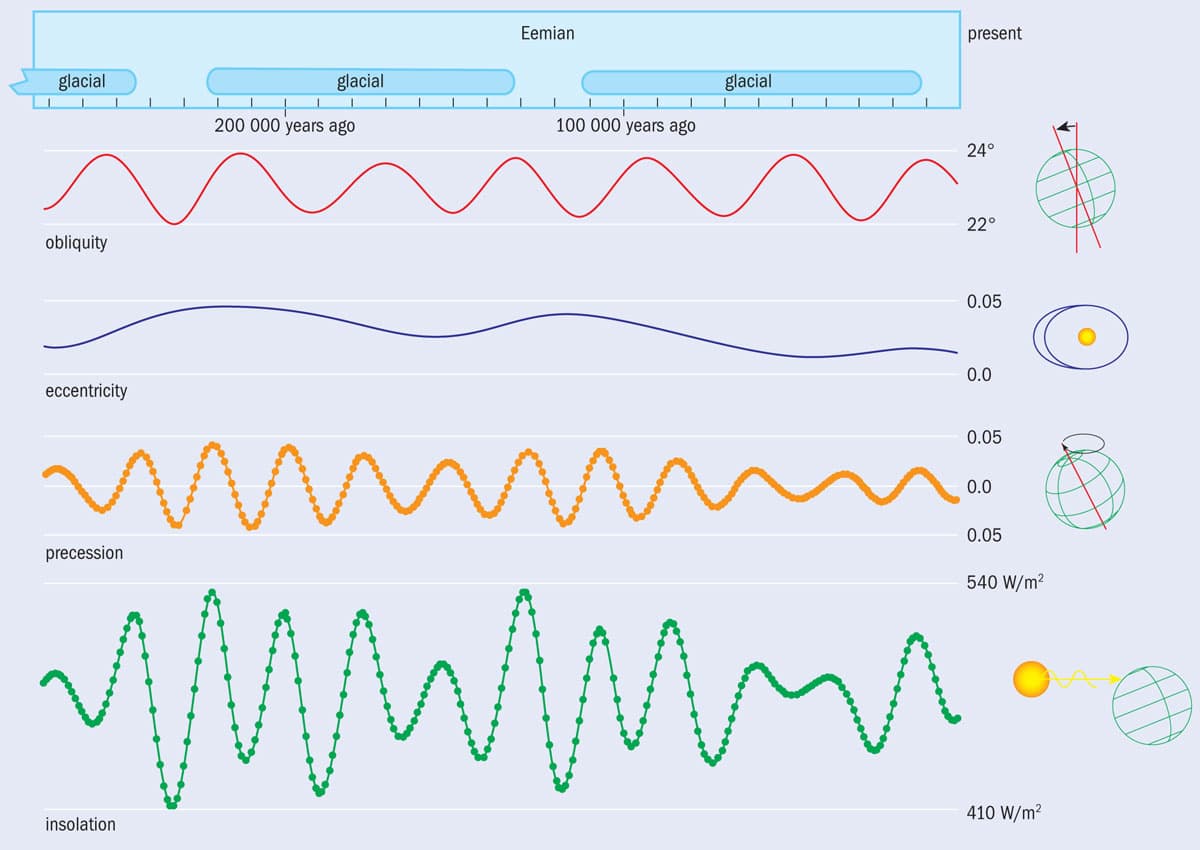
During these cycles, the Earth’s glaciers repeatedly pushed outwards from the poles – sometimes reaching as far as 40˚ either side of the equator – before retreating back and then going out again. Milankovic´ hypothesized that these regular cycles, which reoccurred about once every 110,000 years, were caused by periodic variations in the quantity and distribution of solar radiation falling on the Earth – and that these changes in sunlight were in turn caused by variations in the eccentricity, precession and obliquity of the Earth’s orbit (figure 1).
1 Cycling through history
(Courtesy: Adapted from J Laskar et al. Astronomy and Astrophysics428 261)
As was first realized by the Serbian astronomer Milutin Milankovic´, the Earth has undergone huge climate cycles each lasting roughly 110,000 years during which time the planet’s glaciers repeatedly pushed out towards the equator before retreating. These cycles were caused by periodic variations in the amount and distribution of sunlight falling on the Earth, which were in turn the result of variations in our planet’s obliquity (tilt), eccentricity (deviation from a true circular orbit) and precession (the poles wobbling about the axis). Shown here are the changes in sunlight falling at an altitude of 65°N, given in terms of the rate of energy falling per square metre.
Milankovic´’s ideas remained controversial and for many years remained purely theoretical. But things changed in the 1960s when researchers developed techniques to drill out samples of sediment from the ocean floor – so-called deep-sea cores – and also identified accurate proxies for climate change, particularly the (tiny) changes in the ratio of oxygen-18 to oxygen-16, known as δ18O. As the Nobel-prize-winning chemist Harold Urey and his University of Chicago colleague Cesare Emiliani first showed, the rate at which oxygen-16 is incorporated into a calcium-carbonate crystal lattice depends on temperature, with warmer samples incorporating more. In fact, the situation is more complex: when global temperatures fall and ice sheets grow, the δ18O signal in deep-sea sediments has two parts, one depending on temperature and the other on ice volume.
Thanks in particular to the pioneering work of the University of Cambridge chemist Nicholas Shackleton, measurements of the δ18O ratio in carbonate-secreting Foraminifera micro-organisms have allowed geoscientists to determine how ice sheets in the late Cenozoic era – over at least the last five million years – had periodically grown, melted and then grown again. As a result, it became possible to link the variation in the Earth’s orbit with signatures of δ18O in sedimentary rocks. Shackleton’s work showing that the variation of δ18O in deep-sea cores exactly tracked the astronomical cycles predicted by Milankovic´ was published in a seminal 1976 Science paper written with Jim Hays and John Imbrie called “Variations in the Earth’s orbit: pacemaker of the ice ages” (194 1121).
A better system
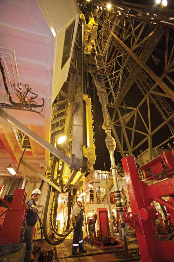
In fact, what had been developed as a way of assessing temperature and ice-volume change in the geological past became so accurate that it morphed into a highly accurate clock for measuring the passage of geological time. As more and more cores from all the world’s oceans were retrieved and analysed – provided the different oxygen isotope “stages” could be unequivocally identified using magnetobiostratigraphy – the astronomical timescale was steadily extended step by step further back in time. This has been achieved with the retrieval of yet more undisturbed cores from the deep sea by researchers working on the Integrated Ocean Drilling Program – an international marine research effort that began in 2003 and that is about to embark on a further 10-year survey. In fact, whereas geologists could previously only date events using astrochronology to those that had happened within, broadly, the last 150,000 years, we can now go back to a quite remarkable 80 million years before the present and it is possible, using astrochronology, to discriminate between events of this antiquity with previously undreamed of resolution.
Deeper and down The Integrated Ocean Drilling Program uses drilling vessels to extract “deep-sea cores” – samples of sea-floor sediment that can be studied by geologists. (Courtesy: IODP)
So accurate has the system become that in 1990 when Shackleton analysed the δ18O signal encoded in a core extracted from the eastern Pacific Ocean, which had a very high sedimentation rate and hence produced thick strata and a good time resolution, he was able to identify one particularly important chron boundary that had occurred 780,000 years ago. Geochronologists had previously assigned it an age of 730,000 years – a difference of more than 6%. Shackleton was so sure about his measurements that he argued that the K–Ar decay constant, which had been used to determine the previous estimate, was incorrect and should be recalibrated. He was right and many geochronologists had to eat humble pie as they had been supplying the geological community with the wrong constant for several years, which meant that much of the rest of the Cenozoic timescale was out too. As one of his graduate students I know, full well, how much Shackleton liked that! He loved nothing better than putting the intellectual cat among the pigeons of scientific consensus and thereafter would often boast of his success over the geochronologists.
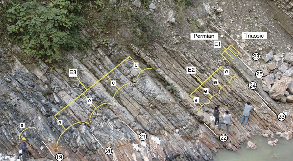
One of the curiosities of astrochronology is that it makes sense of much more of the geological record than just the accurate calibration of the deep-sea record of sediments. “Rhythmically banded” sections – where older rock formations have Milankovic´ cycles imprinted in the form of colour and particle variations – have been found in almost all parts of the geological record from the Late Jurassic epoch (161–145 million years ago) to the Silurian epoch (443–419 million years ago) – as well as much in-between (figure 2). This should mean that in principle the technique can be applied to older sections.
2 Get into the rhythm
(Courtesy: Nature Communications4 2452)
“Rhythmically banded” sections – where older rock formations have Milankovic´ cycles imprinted in the form of colour and particle variations – have been found in almost all parts of the geological record. Shown here is an example of such structures from the Upper Changhsingian Dalong Formation at Shangsi in China, being 252–254 million years old.
Indeed, now that we understand that variations in the Earth’s orbit around the Sun have been such a powerful influence on the record of the past 80 million years of Earth history, it is perhaps not surprising to find that such cycles have affected even earlier times of sedimentary deposition. And yet, all is not straightforward. Although the cycle of glaciations and deglaciations has controlled the oxygen-isotope signal in the deep-sea record over the last 40 million years, the problem is that before then the Earth was ice-free. What then can account for the imprinting of the orbital record on these older cyclic sediments? The probability is that it is the temperature component only, rather than having anything to do with ice volume, particularly at the most sensitive latitudes to incoming solar insolation, which Milankovic´ himself identified as about 65˚N and 65˚S.
And then again, the whole science of astrochronology is based upon the hypothesis that the Earth’s orbital parameters have varied in a uniform and repeatable manner. If these parameters themselves have varied, then some form of correction will need to be devised for any systematic deviations in the astronomically tuned timescale as we delve further and further back into deep time. So next time you find yourself watching George Pal’s version of The Time Machine, with the machine’s endlessly spinning disc, spare a thought for how he correctly, and unawares, saw the future of geology, where time is measured, like his spinning disc, in cycles.
Locusts have been the bane of farmers for centuries. One locust can consume its own body weight in vegetation a day, and in a single plague that struck Ethiopia in 1958, swarms of the insects destroyed 167,000 tonnes of grain – enough to feed a million people for a year. But for the neurobiologist Claire Rind, locusts are also an inspiration. The reason? Their incredible talent for avoiding collisions. Research has shown that locusts can avoid fast-approaching objects as little as 45 ms before a collision – nearly 10 times faster than the blink of a human eye. This ability is crucial to their infamous swarming behaviour: a single swarm can contain millions of insects and may fly 200 km in one day, yet somehow the locusts manage to avoid crashing into each other or triggering airborne mayhem.
After years of studying how locusts react to objects looming towards them, Rind and her interdisciplinary group of collaborators have now used the insects as a model for computerized systems that help robots detect and avoid impending collisions. These systems are based on visual information alone, which is important for two reasons. The first is that they mimic locusts, which, like humans, rely on sight rather than echolocation or the touch of feelers or whiskers to avoid running into things. The other reason why such systems are important is that they could pave the way for quicker-reacting collision sensors and automatic braking systems in cars.
All in the neurons
Rind, a specialist in invertebrate neurobiology at Newcastle University in the UK, began by trying to understand locusts’ amazing ability to avoid collisions. To do this, she and her collaborators took an unusual approach: they made the insects repeatedly watch clips of colliding spaceships from the blockbuster movie series Star Wars. This research earned Rind an Ig Nobel prize for “research that first makes you laugh, and then makes you think” in 2005, but it also revealed that the insects’ visual neurons responded to the looming spacecraft. Later, she discovered that these same neurons triggered escape reactions when flying locusts (as opposed to stationary, cinema-going ones) were approached by objects.
Locusts have several neurons that are “looming-sensitive”, which means that they react to an object that occupies an increasing share of the insect’s field of vision. But the attention of Rind and her team was drawn to a specific pair of neurons called lobula giant movement detectors (LGMDs). Locusts are one of only a handful of species known to have these neurons, and they have two of them – one behind each of their compound eyes, which are located on opposite sides of their bodies. According to Rind’s colleague Roger Santer, this configuration is “particularly cool” because having only one such neuron per locust eye makes it possible to study the same specific neuron in many different locusts. “We can be sure that we are recording from the same neuron in all our experiments, allowing us a good insight into how that particular neuron works,” says Santer, a biologist at Aberystwyth University in the UK.
The group’s studies showed that the LGMD neurons are part of a powerful data-processing system. Fractions of a second before an impending collision, the neuron sends a warning message from the locust’s brain to the motor centres in its wings and legs, triggering immediate evasive action. At first, the locust – like any animal – will instinctively steer out of the incoming object’s way. If it is unable to do so, at the very last moment it “does this emergency last-ditch behaviour that we call a glide”, says Santer. “All of a sudden, it folds its wings up, which we think would cause it to lose height, so at the last moment it drops out of the position where it would’ve been. So if there is an attacking bird that is coming in and wants to grab it, and the locust’s course has suddenly changed, the locust can survive and fly another day.”
Technology mimicking nature
Once the researchers understood how collision detection worked in locusts, they began developing computational models to copy it. One important feature of their model is that it picks out the boundary edges of objects, and then responds only when the rate of the object’s angular change increases (as it would for a rapidly oncoming object). This means that the system detects changes in motion, rather than motion itself – just like the locust, says Rind. However, she adds that her team is still studying the interplay between the locusts’ LGMDs and the neurons’ inputs to determine exactly how it is done biologically.
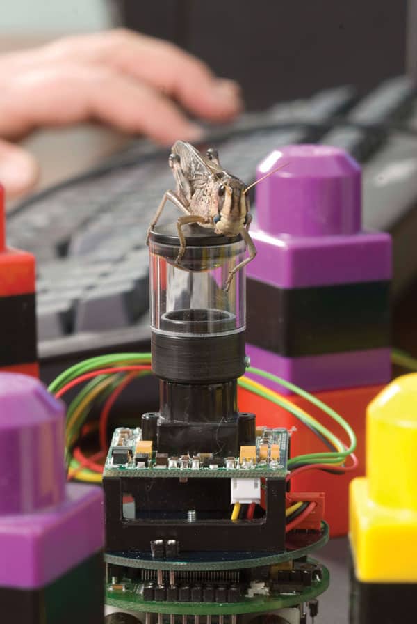
Insipiring ride A locust perches atop one of the robots used in Claire Rind and Shigang Yue’s research. (Courtesy: S Yue and C Rind)
In recent years, Rind and her collaborators have worked with robotics specialist Shigang Yue of the University of Lincoln, UK, to test their computer models with the help of a robot equipped with a miniature video camera and insect-like 360˚ vision. The robot had to find its way along a path full of stationary and moving obstacles, relying on visual input and a combination of two locust-inspired software models to guide its reactions to approaching objects.
In these experiments, output from the video camera was divided into left and right overlapping fields, one for each robotic “eye”. Images from the two fields were then processed by a neural network of simulated cells, the job of which was to react to looming objects and generate motor commands for evasive action. The network consisted of three layers of cells in a so-called “retinotopical” arrangement – meaning that neighbouring cells look at neighbouring areas of the image – plus a fourth “output” cell that summed activity in the layers (a simulated LGMD, in essence).
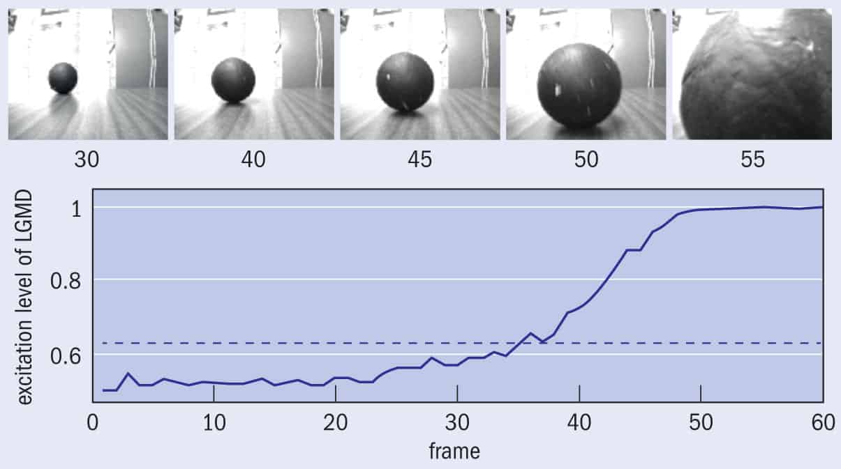
The first layer of cells was composed of photoreceptors, each of them “looking” at a small region of the video image. When the approach of an object’s edge caused the level of light falling onto a photoreceptor to change, the cell sent a signal to its counterpart in the same retinotopic position in the second layer of cells. Excitation from the signal also generated a “ring of inhibition” in the third layer that spread out like ripples on a pond, creating an inhibitory area, or mask, around the excitation. This was important because when an object approaches, both the amount of edge and the speed of the edge’s movement on the photoreceptors’ surface increase exponentially. Hence, the faster the edges move, the more likely it is that the excitation they cause can jump over the inhibited cells onto ones that are not yet inhibited, and are thus able to react and transmit excitation. This then allows excitation to build up in the simulated LGMDs (figure 1), and the final step is to convert their output into motor commands that would cause the robot to brake and move to avoid running into things.
The results were impressive: the group’s robot could perceive an imminent collision and avoid it in 500 ms – not quite as fast as a blink of a human eye, which is typically over within 400 ms, but still promising for a new method. “The system works because it extracts features of images that are most indicative of collision, such as edges that move with increasing angular velocity over the facets of the compound eye,” Rind explains. “Edges that move with the same velocity or a decreasing velocity cannot effectively trigger a warning. The system is used at different sensitivities, so the sudden presence of an object triggers one type of reaction whereas an object that would cause an imminent interception – in the locust’s case, a bird such as a black kite that catches locusts in a swarm, a metre or so away, triggers another.”
1 Looming large
(Courtesy: Adapted from IEEE Trans. Autonomous Mental Dev.5 173)
In this test scene from Claire Rind and Shigang Yue’s research, a ball was sent rolling towards a robot equipped with a video camera and an “LGMD agent” – a network of simulated cells that mimics the image-processing techniques of a locust’s neurons. As the ball loomed larger in the robot’s field of view (see series of images above), excitation levels in the simulated LGMD increased, reaching a threshold (blue dashed line) between frames 30 and 40 and peaking shortly before impact in frame 55. Video footage was recorded at about 25 frames per second.
From swarms to traffic jams
In Rind’s view, the collision-avoidance system that evolved in the locust and that her team has mimicked in a robot is better than the conventional radar- or infrared-based collision-avoidance systems currently used in autonomous cars. As well as being more complex (and potentially more expensive), these other methods also rely on very heavy-duty computer processing, and do not react well to sudden changes (such as a child running onto the road) or cluttered environments containing many people and vehicles.
This solution copied from biology is potentially simpler and more efficient than conventional computer vision approaches
Noel Sharkey, an artificial intelligence and robotics researcher at the University of Sheffield, UK, who was not involved in Rind’s research, agrees that if the locust-mimicking system were incorporated into an autonomous car, it would likely perform better than other vision-based systems for collision avoidance. However, he adds, most autonomous vehicles currently in development use sonar sensors, which are also extremely fast and not too costly. Another researcher, bioroboticist Barbara Webb of the University of Edinburgh, UK, points out that the system would need to be tested at car-like speeds, under road-like conditions, and over long distances before it could be incorporated into an autonomous vehicle. Still, she adds, “This solution copied from biology is potentially simpler and more efficient than conventional computer vision approaches, hence more useful for applications such as robots and cars.”
Although a car with a locust-inspired collision-avoidance system may still be some way off, Rind’s colleague Yue notes that artificial visual neural systems could also provide new solutions for computer vision in other dynamic environments, such as helping people who are visually impaired or improving the movements of non-player characters in video games. Rind, meanwhile, is optimistic about her system’s chances of finding its way to a highway near you. “Our system is not implemented anywhere yet, but as our economy and others pick up, motor manufacturing will have more money to spend on innovative safety measures,” she says. “Public pressure to have safer cars is a good motivator.”
In less than 100 seconds, John Dainton argues the importance of giving academics the freedom to explore their intellectual curiosities. Many huge developments to benefit society – including the electrification of technologies and the World Wide Web – have emerged from the pursuit of fundamental answers, Dainton explains.
Just in time for Christmas, researchers at the Massachusetts Institute of Technology (MIT) have unveiled the ultimate “cocktail accessory”. It’s an edible self-propelled boat that whizzes around on the surface of an alcoholic drink.
Researchers in the US have observed room-temperature ferromagnetism in a graphene nanostructure for the first time. The result, until now only predicted by theory, suggests that graphene could be used to create spintronics devices, which are circuits that use the spin of the electron to process and store information.
Graphene, a sheet of carbon just one atom thick, is a promising material for making molecular electronic devices of the future thanks to its unique electronic and mechanical properties. These include extremely high electrical and thermal conductivity plus exceptional mechanical strength. Room-temperature ferromagnetism can now be added to this already impressive list.
Sakhrat Khizroev at Florida International University and colleagues made their discovery by making a number of different measurements of the magnetic properties of graphene samples that had been functionalized with nitrophenyl (NP) groups. This involves the attachment of NP groups to the surface of graphene (see figure). The resulting graphene-based material appears to become an organic molecular magnet with ferromagnetic and antiferromagnetic ordering that persists at temperatures above 400 K.
“Unpairing” electron spins
The researchers, who include Jeongmin Hong at the University of California, Berkeley, Robert Haddon at University of California, Riverside and Walt de Heer at the Georgia Institute of Technology, have been working on these experiments since 2008. “We believe that the NP groups act to unpair electron spins at periodically spaced carbon sites along certain graphene orientations, known as ‘armchair’ and ‘zigzag’,” Hong says. “It is the interactions between these unpaired spins that lead to the magnetic order we observed.” Graphene functionalized with hydrogen also appears to have similar magnetic properties, he adds.
Ours is a “gentle chemistry” approach
Jeongmin Hong of the University of California, Berkeley
“Ours is a ‘gentle chemistry’ approach that makes use of functionalization rather than introducing defects into graphene, which is a much more aggressive strategy,” Hong explains. “Although previous research mainly looked at heavily defected material, large numbers of defects in graphene can hinder the formation of the pure zigzag edges needed for magnetism here.”
According to the researchers, the NP-functionalized graphene could be used as a new type of single-layer magnet. It might also be used to make new types of spintronics devices based entirely on carbon that exploit the unpaired spins that are present. Spintronics is a relatively new technology that exploits the spin of an electron as well as its charge.
More details about the research can be found in ACS Nano.
Not many school pupils can boast having had a world-champion physics teacher, so say hello to Julie McGavigan, who teaches physics at Eastwood High School near Glasgow and bagged a gold medal at the World Karate Championships in Denmark in October.
The 27 year old, who says the win in Denmark came as “quite a shock”, is a 3rd Dan in Shotokan karate and has taught physics for five years after studying the subject at the University of Glasgow.
McGavigan also teaches karate at evening classes at Eastwood High, where she puts physics principles to good use. “Physics helps me understand why certain stances, moves and combinations work when practising karate,” McGavigan told physicsworld.com.
“Wizzing” to the top of the Red Folder this week is a group of physicists at the “Splash Lab” at Brigham Young University who have studied the physics of “splashback” that occurs when people urinate. Using high-speed cameras the researchers filmed jets of liquid from a “synthetic urethra” striking toilet walls. They found that the stream of liquid breaks up into droplets when it is about 15 cm from the urethra exit. “Wizz kids” Tadd Truscott and Randy Hurd suggest that apart from sitting down on the toilet (and risk being called Sitzpinklers by their German friends), men should get nice and close when doing their business to eliminate splashback. Take a look at their video about “Urinal dynamics” above.



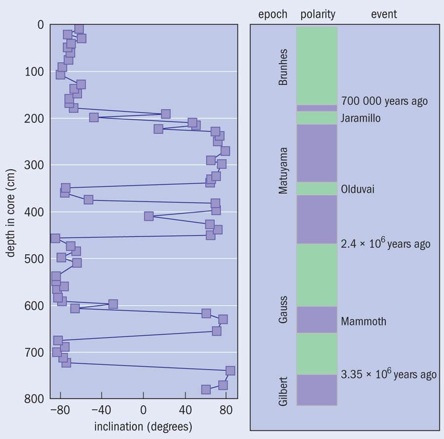 It has been known since the 1920s that the Earth’s magnetic field undergoes periodic reversals, with the most recent of these zones of flip-flopping magnetism (“chrons”) depicted on the above timeline. (Green indicates that the direction, or “inclination”, of the field was opposite to what it is today.) The rocks that were being created in the regions where new crust forms (mid-ocean ridges) took on the magnetization prevailing at the time. These rocks are formed where tectonic plates move apart and lava emerges from the gap between the plates before spreading horizontally along the sea-bed floor. But the magnetic field directions are also encoded at different depths in sediments below the sea bed. So as the sea bed spreads at a more-or-less constant rate of about 1 cm per 1000 years, if you can measure the horizontal distance between chrons on the sea bed it is possible to estimate the time that elapsed between magnetic reversals. And if you match the age of a recently formed region on the sea floor with its corresponding chron in a sediment, you can start assigning dates to chrons – and hence to biostratigraphic boundaries calculated by studying the fossil record.