Are dusty quasars masquerading as Dyson sphere candidates?

Seven candidate Dyson spheres found from their excess infrared radiation could be a case of mistaken identity, with evidence for dusty background galaxies spotted close to three of them.

The seven candidates were discovered by Project Hephaistos, which is coordinated by astronomers at Uppsala University in Sweden and Penn State University in the US.

A Dyson sphere is a hypothetical construct: a swarm of energy collectors capturing all of a star’s radiant energy to provide huge amounts of power for its builders. As these energy collectors – basically huge arrays of solar panels – absorb sunlight, they must emit waste heat as infrared radiation to avoid overheating. While a complete Dyson swarm would hide a star from view, this waste heat would still be detectable.

The caveat is that to build a complete Dyson swarm, a lot of raw material is required. In his 1960 paper describing the concept, Freeman Dyson calculated that dismantling a gas giant planet like Jupiter should do the trick.

Given that this is easier said than done, Project Hephaistos has been looking for incomplete Dyson swarms “that do not block all starlight, but a fraction of it,” says Matías Suazo of Uppsala University, who is leading the project.

Suazo’s team searched five million objects in archival data from NASA’s Wide-field Infrared Survey Explorer (WISE) and Two Micron All-Sky Survey (2MASS), and cross-checked them against photometry and distance data accrued by the European Space Agency’s Gaia mission. This resulted in seven candidates exhibiting a suspicious infrared excess, as reported in Monthly Notices of the Royal Astronomical Society.

All the candidates are M-dwarfs, which are the smallest, coolest and most common type of star in the Universe. The closest is located 466 light years away.

Debris discs and Hot DOGs

Yet questions have now arisen over the real nature of these candidates.

“They could be an astrophysical phenomenon such as extreme debris discs, or something more exotic,” says Ann Marie Cody, an astronomer at the SETI Institute in California who is not involved in Project Hephaistos, but has conducted her own Dyson swarm search. “However, the data published thus far cannot discriminate between these scenarios.”

Debris discs are the dusty remnants of planet formation, but while many M-dwarfs have been found to have planets, only a handful have been found with sizeable debris discs, leading Suazo to be sceptical of the debris disc explanation.

“Observationally, M-dwarf debris discs are really uncommon,” Suazo tells Physics World. “There are different theories about why, including observational biases, formation mechanisms and so on. Those few cases that have been confirmed are in the submillimetre/radio regime, which means they are way cooler than the temperature range of our models.”

Tongtian Ren and Michael Garrett of the Jodrell Bank Centre for Astrophysics at the University of Manchester, and Andrew Siemion of Breakthrough Listen and the University of Oxford, have proposed that the candidates have another explanation: background contamination from distant, dusty quasars.

They found strong radio sources very close in the sky to three of the candidates. Each radio source is attributed to an active supermassive black hole at the centre of a very distant, dusty quasar known as a “Hot DOG”, or hot dust-obscured galaxy. Because they are dusty, they radiate infrared and are large enough in the sky to extend behind the Dyson swarm candidates.

Although no coincident radio sources were found near the four remaining candidates, the density of Hot DOGs in the sky leads Ren, Garrett and Siemion to conclude that they most probably are also contamination from Hot DOGs, but ones that are radio quiet.

But Garrett isn’t completely ruling out Dyson swarms.

“We still think the sources are worth pursuing with new observations across the electromagnetic spectrum to see which interpretation is correct,” he tells Physics World.

JWST to the rescue?

More bad news for the candidates comes from Cody’s Dyson swarm search, which used NASA’s Transiting Exoplanet Survey Satellite (TESS) to look for anomalous transits that could potentially signpost large, artificial structures.

“Our optical photometry pipeline did not classify the Dyson sphere candidates as having any anomalous variability,” says Cody. “In fact, I personally examined the available TESS data for each of the seven objects in this paper, and none of them appear to be significantly variable.”

To settle the matter, Suazo, Garrett and Cody all agree that spectroscopic observations are now vital. If dust is present, either in a disc or a background galaxy, it would produce specific absorption lines. Alternatively, spectroscopy could measure the energy distribution of a candidate star’s photosphere (its visible surface) so that a best-fit model can be applied to determine whether a candidate really is consistent with a Dyson swarm.

“James Webb Space Telescope data would be ideal, since it could quickly rule out or confirm the debris disc or the galaxy contamination explanations,” says Suazo.

If the Hot DOGs explanation turns out to be correct, it leaves the hunt for Dyson swarms in a difficult place. An infrared excess is a Dyson swarm’s calling card, but if contamination from background galaxies is the probable answer each time, how can one distinguish artificial megastructures from natural phenomena?

“It’s a good question,” says Garrett. “Hot DOGs would be detected in deep near-infrared observations. There might also be some subtle aspects of the data that would be a tell-tale sign of contamination – we will start looking at that now.”

Having already probed 60 million stars, Cody’s search continues and her team is still vetting about a thousand events that are probably eclipsing binaries, but you never know.

For Cody, a multifaceted approach is essential in hunting for Dyson swarms. “With photometric data alone, it can be challenging to distinguish between rare astrophysical phenomena and Dyson swarms,” she says. “However, I believe that optical and infrared spectroscopic data may assist with the task.”

Early Earth’s magnetic field strength was similar to today’s

Ancient organisms preserved in the Earth’s oldest fossils may have experienced a planetary magnetic field similar to the one we observe today. This finding, from a team of researchers at the University of Oxford, UK and the Massachusetts Institute of Technology in the US, suggests that the planet’s magnetic field was relatively strong 3.7 billion years ago – a fact with important consequences for early microbial Earthlings.

“Our finding is interesting because the Sun was generating a much more intense solar wind in the Earth’s early history,” explains team leader Claire Nichols of Oxford’s Department of Earth Sciences. “This means that the same strength of magnetic field would have provided far less shielding (because the protective ‘bubble’ around Earth provided by the magnetosphere would have been much smaller) for life emerging at that time.”

Without the magnetosphere, which protects us from cosmic radiation as well as the solar wind, many scientists think that life as we know it would not have been possible. Until now, however, researchers weren’t sure when it first appeared or how strong it was.

Unique rock samples

In the new work, Nichols and colleagues analysed rocks from the northern edge of the Isua Supracrustal Belt in southwest Greenland. Billions of years ago, as these rocks were heated, crystals of magnetite formed, and iron oxide particles within them recorded the strength and direction of the ambient magnetic field.

While similar processes happened in many places and at many times during Earth’s history, the rocks in the northernmost part of Isua are extremely unusual. This is because their location atop a thick continental crust prevented their magnetic information from being “erased” by later geological activity.

Indeed, according to the researchers, this band of land experienced only three significant thermal events in its history. The first and hottest occurred 3.7 billion years ago and heated the rocks up to 550 °C. The two subsequent heating events were less intense, and because they did not heat the rocks to more than 400 °C, the 3.7-billion-year-old record of Earth’s magnetic field remains as it was after the first event locked it in.

Recovering a vector of magnetization

Collecting samples from Isua was challenging, Nichols says, because the sample site is so remote it can only be reached by helicopter. Once back in the laboratory, the team demagnetized the samples stepwise, either by gradually heating them or by applying increasingly strong alternating magnetic fields. “These processes allow us to slowly remove the magnetic signal from the samples,” Nichols explains, “and recover a vector of magnetization that tells us about the direction of the ancient magnetic field.”

To determine the strength of the ancient field, the researchers applied a known magnetic field and compared the vector of magnetization acquired in the lab to that recovered in the original demagnetization. They found that rocks dating from 3.7 billion years ago recorded a magnetic field strength of at least 15 microtesla (µT). To compare, Earth’s present-day magnetic field averages around 30 µT. These results constitute the oldest estimate of the Earth’s magnetic field strength ever recovered from bulk rock samples – a method that is more accurate and reliable than previous analyses of individual crystals.

Consequences for early life

The fact that the Earth’s magnetic field was already fairly strong 3.7 billion years ago has several implications. One is that, over time, as the solar wind decreased, life on Earth would have become progressively less likely to experience high levels of ionizing radiation. This may have allowed organisms to move onto land and leave the more protective environment of the deep oceans, Nichols says.

The results also suggest that Earth’s early magnetic dynamo was as efficient as the mechanism that generates our planet’s magnetic field today. This finding will help scientists better understand when the Earth’s inner, solid core began to form, potentially shedding light on processes such as mantle convection and plate tectonics.

Are magnetic fields a key criteria for habitability?

Perhaps the most profound implication, though, concerns the possibility of life on other planets. “Understanding the oldest record of Earth’s magnetic field is really important for figuring out whether magnetic fields are a key criteria for habitability,” Nichols tells Physics World. “I’m really interested to know why Earth appears so unique – and whether the magnetic field matters for its uniqueness.”

The technique developed in this study, which is detailed in the Journal of Geophysical Research, could be used to study other very old rocks, such as such as those found in Australia, Canada and South Africa. Nichols says her next big project will be to carry out similar studies on these rocks.

Blurred tomography fabricates custom microlenses with optically smooth surfaces

Additive manufacturing, also known as 3D printing, has revolutionized many sectors with its speed, flexibility and unparalleled design freedom. But previous attempts to create high-quality optical components using additive manufacturing methods often came up against a range of obstacles. Now, researchers from the National Research Council of Canada have turned to blurred tomography – an extension of the tomographic volumetric additive manufacturing (VAM) method – to create customized optical components.

“3D printing is transforming every sector of manufacturing,” says lead author Daniel Webber. “I’ve always been interested in 3D printed optics due to their potential to revolutionize optical system design. I saw a post-doc position with the NRC where they wanted to do volumetric 3D printing of micro-optics, and the rest was history”.

Additive manufacturing challenges

In the past, techniques such as digital light processing, stereolithography, inkjet printing and two-photon polymerization (2PP) have been used to build optical components through a layer-by-layer approach. However, the fabrication process tends to be slow, it’s difficult to fabricate optical components with curvature – which many components need – and surfaces that aren’t parallel to the substrate have height steps defined by the layer thickness.

VAM has also had its challenges, with poor part quality (such as ridges on the surface called striations) due to the self-writing waveguide effect – in which the narrow writing beams used in VAM cause increased printing speed in planes parallel to the beams. Post-processing methods are usually required to increase the part quality and smooth the surfaces, but a direct VAM method that doesn’t require extra steps has been sought.

Overcoming challenges with blurred tomography

In their latest research, Webber and his team have accomplished such a direct VAM method, while maintaining the freedom of design that additive manufacturing offers for rapid prototyping.

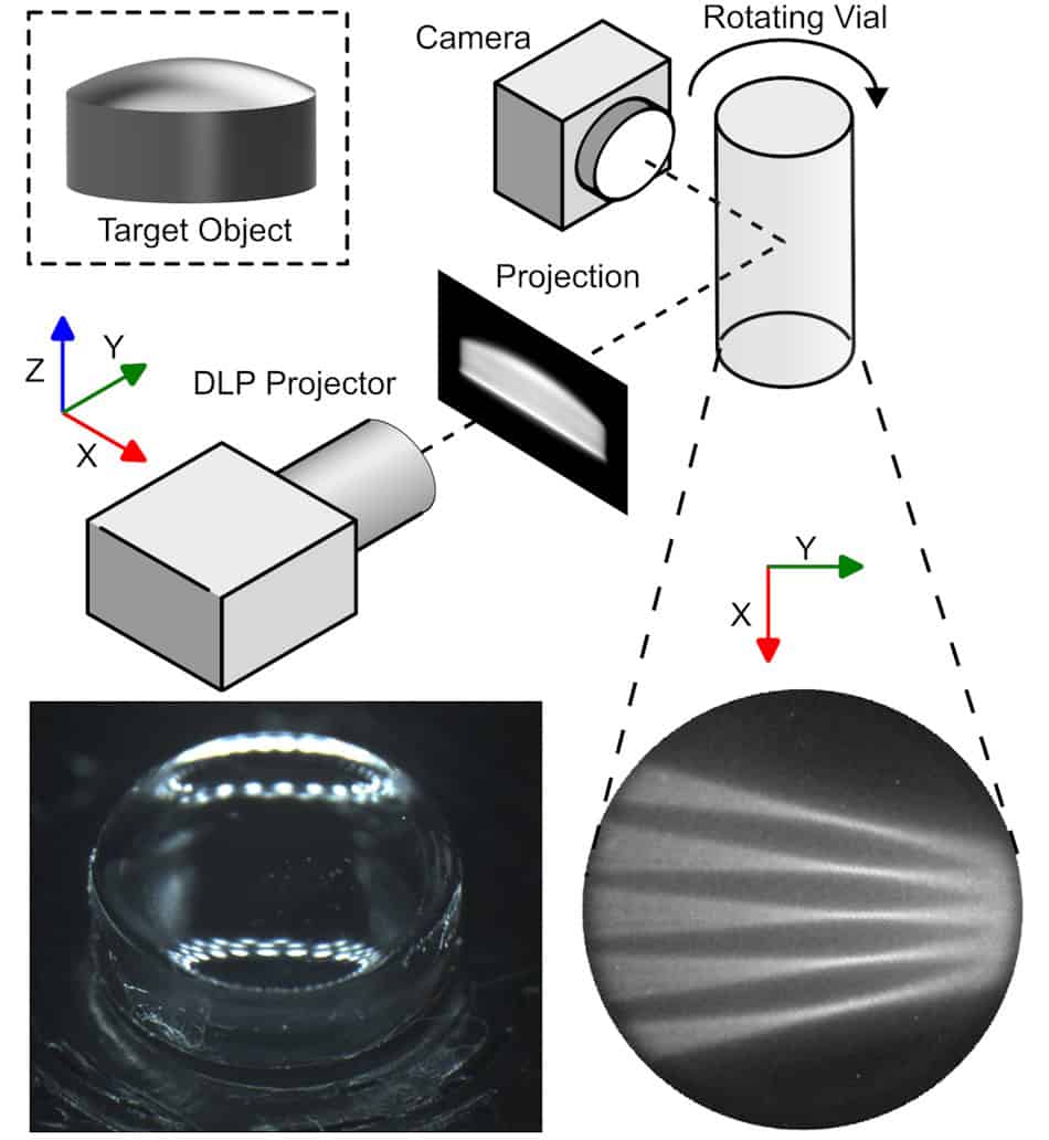
Tomographic VAM uses projected light to solidify a photosensitive resin in specific regions, enabling parts to be built without support structures. While the pencil-like beams used in conventional tomographic VAM methods cause striations, the new technique can produce microlenses with commercial-grade quality. It is known as blurred tomography, because a large-etendue (more “spread out”) source is used to purposely blur the lines and reduce striations.

The blurring of the optical writing beam helped to generate a surface roughness in the sub-nanometre range – making it essentially molecularly smooth. By comparison, other VAM methods have well-collimated and low-etendue writing beams so that they are not blurred by design.

3D printing setup

By purposely blurring the beam and coupling it with astigmatism introduced by the cylindrical vial of photoresin (without an index matching bath), the blurring could be achieved across the whole print volume. Alongside the rapid processing speed, the other defining feature of the blurred tomography method is that it doesn’t require additional processing and is therefore a direct method for producing smooth optical components.

“The most significant finding of this work is that we can directly fabricate optically smooth surfaces and have freeform ready-to-use optical components in under 30 minutes,” says Webber.

While the overall processing time takes around 30 min, the actual printing of the lenses took less than a minute. This is similar to other VAM techniques (but without the need for extra surface processing steps). In comparison, a previous study found that using 2PP to print a half-ball lens of similar size (2 versus 3 mm), curvature error (3.9% versus 5.4%) and surface roughness (2.9 versus 0.53 nm) took 23 h – showing how blurred tomography is much faster, while producing finer surface features.

The research team showcased the potential of the new technique by making a millimetre-sized plano-convex optical lens with an imaging performance comparable to that of a commercial glass lens. The intrinsic freedom design that additive manufacturing offers also helped the researchers create a biconvex microlens array (fabrication on both sides), as well as overprinting of a lens onto an optical fibre.

Like many areas of additive manufacturing, it’s thought that VAM could offer a way of producing low-cost and rapidly prototyped parts, in particular, freeform optical components. “We have demonstrated that blurred tomography is capable of rapidly fabricating a range of micro-optical components. Moving forward, we would like to extend these capabilities to larger part sizes and new materials,” Webber tells Physics World.

The research was published in Optica.

Ion therapy, mass spectrometry and the origins of life: Lily Ellis-Gibbings shares her passion for creating novel instrumentation

How did you first become interested in working in the field of instrumentation?

When I was in the final year of my bachelor’s degree in Australia I was looking for an undergraduate project and the one I chose involved studying atomic and molecular collisions. This meant working with homemade vacuum equipment and instrumentation, which I really liked. I discovered that I really enjoy doing experiments that take an incredibly complicated physical system and break it down into smaller and smaller pieces – until your measurements reveal something fundamental about the system you are studying.

After I graduated, a friend and I went on a road trip to visit universities and chat with potential PhD supervisors. However, I couldn’t find a good fit, so I worked for a few years as a science communication officer.

That was a really great experience, but after a while I was looking for something more scientific and a little more challenging. The professor that I did the undergraduate project with had a colleague in Spain who was looking for someone to do a PhD in a similar field. So I was very lucky to be in the right place at the right time – and to have some experience in vacuum instrumentation.

Your PhD at the Autonomous University of Madrid involved the development of new ion sources for radiotherapy. What was the goal of that research?

The focus was on ion therapy, which is a type of cancer treatment that uses a high-energy beam of protons, or perhaps carbon ions, to destroy a tumour within the body. Ions are particularly good at this application, because, due to an effect called the Bragg peak, the beam can be adjusted to deposit most of its energy in the tumour – minimising damage to the healthy tissue that it must pass through to reach the tumour.

It turns out that it’s not just the high-energy ions that affect the tumour. Ion collisions create a cascade of lower energy particles such as electrons and free radicals. These can affect tumour cells in lots of different ways – sometimes even killing the cells.

We were trying to develop ion sources that could mimic the secondary particles created when an ion beam interacts with molecules in the body. In particular, we were interested in how these ions interact with DNA, proteins and other complex molecules. This builds more complex computer models of ion therapy, whereas many conventional models use a body that is modelled as being 100% water.

After you completed your PhD, you worked in experimental astrochemistry at University College London, that must have been a fascinating field to be involved with.

Yes, astrochemistry is a super fun field and I really enjoyed it. It is the study of the chemistry that occurs in different parts of space. Although it sounds very different to my work in radiotherapy, there were similarities in terms of the instrumentation that we used – specifically ion and electron beams in vacuum systems. We focused on how these beams interacted with molecules of astrochemical interest. For example, if a molecule is detected in the ionosphere of Saturn’s moon Titan we could study how that molecule could break down in that environment and form new bonds. Could it turn into singly charged or a doubly charged ion?

Have you studied molecules that may be involved in the emergence of life?

That is certainly something we were interested in. Abiogenesis, the process by which life emerged from non-living matter, is an important topic in astrochemistry. Indeed, one of the reasons we would choose certain molecules to investigate is their possible roles in the emergence of life. For example, I would work with molecules that have carbon–nitrogen bonds because these bonds are really important in how we believe life first appeared on Earth.

That sounds like an exciting field, did you enjoy it?

It was fun and I definitely learned a lot. The astronomy conferences were fascinating and I loved seeing the amazing images that were created from telescope data. The overlap between people doing astrochemistry and the observational astronomers was fairly small. But, we did interact a lot with a lot of physicists who model what the concentrations of different atoms in different parts of the universe should be. It was fascinating speaking with them.

NPL Reception

You joined NPL in 2021, where you are a higher scientist. What does your job entail?

I joined the National Centre of Excellence in Mass Spectrometry Imaging (NiCE-MSI) at NPL in Teddington, London. We mostly work on the chemical imaging of surfaces and a lot of what we do is focused on biology. The measurements that we make are different from what I did before, but again, the instrumentation is similar.

In mass spectrometry imaging we use many different ion sources, some of which operate at high vacuum. But, the really cool thing that I am doing at the moment is the development of ambient ion sources. Conventional mass spectrometry imaging involves ionizing samples under vacuum conditions, often with a lot of sample preparation. However, some components or types of samples – particularly in delicate or unusual biological samples – cannot be studied fully in this way.

Our group ensures that mass spectrometry techniques are quantifiable and repeatable

To address this problem, I’m developing ambient ionization techniques that allow us to do mass spectrometry on samples in air with no sample preparation. I particularly enjoy working with unusual sample types such as plant matter. It’s interesting work and there are always new challenges.

NPL is very involved in developing measurement standards, so our group ensures that mass spectrometry techniques are quantifiable and repeatable. It is important that we maintain our high level of scientific integrity that we have within the metrology (measurement science) community.

Do you work with researchers outside of NPL?

Yes, we have extensive collaborations across the UK. We recently partnered with Cancer Research UK on a project called Rosetta, which involves using mass spectrometry imaging to map cancer biology. We also collaborate with the Rosalind Franklin Institute in this field and we partner with researchers based at universities around the UK. We contribute our experimental expertise to these projects and we are also involved in analysing data gathered by the collaborations.

NPL also takes part in collaborations with other metrology institutes around the world, including the National Institute of Standards and Technology (NIST) in the US.

What advice do you have for a physics PhD student who would like a career in instrumentation?

Try to spend as much time in the lab as you can. Fix things that are broken, with the appropriate guidance. Work-out how the electronic equipment in your lab works and be hands-on when it comes to tasks like putting together a vacuum system. It’s also important that you learn how to use computer-aided design (CAD) software and understand machine engineering basics – this will allow you to design, commission and build your own equipment.

One thing that I found very useful, is learning how to assemble and disassemble delicate equipment using tiny tools while wearing gloves. Through hours of practice, I taught myself not to be clumsy and to organize parts and tools so I don’t lose them.

One thing that is important to realize is that building instrumentation as an academic scientist can be risky. If you work on a project that fails to deliver data and publications, it can be very difficult when applying for the next job or fellowship. It’s always good to have a side project that trundles along and also produces data – so you always have something you can publish.

What about a career outside of academia?

Scientific institutes, like us at NPL, often mix academic, commercial and measurement services. There are also lots of companies that produce scientific instrumentation and they employ some really amazing scientists. So, that is an excellent career path.

Quantum error correction produces better ‘magic’ states

Humans like to build robust systems – ones that resist change and minimize unreliable or undesirable results. In quantum computing, this desire manifests itself as fault-tolerant quantum computing (FTQC), which aims to protect both the quantum state and the logic gates that manipulate it against interventions from the environment. Although quite a resource-intensive task, physicists at IBM Research recently showed that they could partially meet this requirement, thanks to some real-life quantum “magic”.

The process of cushioning quantum states against uncontrollable interventions is called quantum error correction (QEC). In this process, information that would ideally be stored in a few quantum bits, or qubits, is instead stored in many more. The resulting redundancy is used to detect and correct the enforced errors. In QEC jargon, the mapping of the ideal-case quantum state (the logical state) into the noise-protected state (the physical state) is termed encoding. There are multiple ways to perform this encoding, and each such scheme is called an error-correction code.

FTQC begins with QEC as a first step and then uses appropriate encoded gates and measurements to robustly perform a computation. For it to succeed, the error rate must fall below a certain threshold. Achieving this low error rate remains a significant challenge due to the huge number of physical qubits required in the aforementioned encodings. However, researchers are making significant improvements to FTQC sub-routines.

A little bit of magic

One such improvement recently came from an IBM team led by Maika Takita and Benjamin J Brown. In this work, which is published in Nature, the team proposed and implemented an error-suppressing encoding circuit that prepares high-fidelity “magic states”. To understand what a magic state is, one must first recognize that some operations are much easier to implement in FTQC than others. These operations are known as the stabiliser or Clifford operations. But with these operations alone, we cannot perform useful computations. Does this render Clifford circuits useless? No! When a class of states called magic states is injected into these circuits, the circuits can do any computation that quantum theory permits. In other words, injecting magic states introduces universality into Clifford circuits.

The next important question becomes, how do you prepare a magic state? Until a few decades ago, the best techniques for doing so only created low-quality copies of these states. Then, two researchers, Sergey Bravyi and Alexei Kitaev, proposed a method called magic state distillation (MSD). If one starts with many qubits in noisy copies of magic states, MSD can be used to create a single, purified magic state. Crucially, this is possible using only Clifford operations and measurements, which are “easy” in FTQC. Bravyi and Kitaev’s insight created a leading FTQC model of computation called quantum computation via MSD.

Of course, one can always start with a circuit that allows for operations outside the Clifford set. Then no input state remains “magical”. But the big advantage of sticking to Clifford circuits supplemented by magic states is that its universality reduces the general fault-tolerance problem to that of performing fault-tolerant Clifford circuits only. Moreover, most known error correcting codes are defined in terms of Clifford operations, making this model a crucial one for near-future exploration.

High fidelity of states

While MSD requires a large number of attempts to prepare the intended state, the IBM researchers showed that these can be reduced by preparing input magic states (to MSD) with high fidelity – meaning that the states prepared are very close to those required. In a proof-of-concept demonstration, the IBM team prepared an encoded magic state that is robust against any single-qubit error. Using four qubits of the 27-qubit IBM Falcon processor on the ibm_peekskill system to encode the controlled-Z (CZ) magic state, they achieved fidelities equivalent to the square of the fidelity they would have achieved without encoding the initial state.

The team also improved the encoded state’s yield – that is, the number of magic states produced over time – by introducing adaptivity, which is where mid-circuit measurement outputs are fed forward to choose the next operations needed to reach the required magic state. “Basically, we can create more magic states and less junk,” says team leader Benjamin Brown, who holds appointments at IBM Quantum’s T J Watson Research Center in New York, US and at IBM Denmark.  Both these observed advantages, in yield and fidelity, are due to quantum error correction that suppresses the noise accumulated during state preparation.

Verifying the states prepared

The team verified that they had created the intended magic state (and hence the claimed gain in the fidelity) via tomography experiments. In one experiment, the fault-tolerant circuits measure the physical state in such a way that only the information about the logical state is revealed. This is termed logical tomography. Meanwhile, the other experiment, called physical tomography, determines the exact physical state. As might be expected, logical tomography is more efficient and requires fewer resources than physical tomography. For example, in the case of the CZ state, the former required 7 while the latter required 81 measurement circuits.

As well as demonstrating the advantage of quantum error correction, the new work also opens up a new research pathway – invoking adaptivity to prepare high-fidelity, high-yield magic states with further important implications in developing creative fault-tolerant computing techniques. “This experiment sets us on the path to solving one of the most important challenges in quantum computing – running high-fidelity logical gates on error-corrected qubits,” Brown says.

Boson sampler uses atoms rather than photons

A boson sampler that uses atoms rather than photons has been developed by researchers in the US. The team used its system to determine a complex quantum state more accurately than would be practicable using a conventional (classical) computer. Atoms interact much more strongly than photons, so the researchers believe their system is a promising platform for simulating condensed-matter systems. Looking further in the future, it could also be used for quantum computing.

A defining property of bosons is that an unlimited number can occupy the same state at any one time. This leads to strange behaviour such as the Hong-Ou-Mandel effect, in which two indistinguishable photons striking a 50:50 beamsplitter at the same instance will always come out of the same port. Similar effects involving multiple photons and beamsplitters are extremely difficult for classical computers to model. The best classical algorithms can only manage around 50 bosons.

Boson sampling machines are proto-quantum computers, or quantum simulators, that utilize the properties of bosons themselves. A specific quantum state is imprinted into the system at the input and the state is measured after a given time. However, photons are easily lost in a system, making it very challenging to achieve a reliable measurement.

Square optical lattice

In the new work, researchers in Adam Kaufman’s group at JILA in Boulder, Colorado implemented a boson sampler using atom optics. They placed 180 strontium-88 atoms into a 48×48 site square optical lattice potential. Key to their success, the researchers used an optical tweezer array to move atoms around. Aaron Young, then Kaufman’s PhD student, explains: “We worked hard in this experiment to engineer the tweezers to really address single lattice sites. Our tweezers are smaller than typical tweezers.”

Once the researchers had placed the atoms appropriately, they turned off the tweezers. They then laser cooled the atoms and imaged the initial quantum state. Next, they reduced the depth of the lattice potential, allowing atoms to tunnel between sites. After allowing the state to evolve for a fixed time, they increased the potential depth again, tightly confining the atoms and thereby allowing them to image the positions of the atoms using photons.

The next step was to test the system, explains Young. “Certification of a boson sampler is believed to be as hard as simulating a boson sampler in the first place”. As it is not possible to simulate a boson sampler of 180 indistinguishable atoms classically in a reasonable amount of time, nor is it possible to check whether or not such a boson sampler produced the correct result. The researchers therefore turned to indirect certification by looking at cases in which the bosons were not indistinguishable. Such a state might arise in an experiment as a result of imperfect cooling, for example.

Distinguishable atoms

“As we make the atoms more and more distinguishable, we go from this problem that’s really hard to simulate closer to the case where you’re doing the one atom problem 180 times,” says Young. “And somewhere in the middle we cross the threshold where it’s once again possible to simulate our problem on a normal computer. We check two things: first, that as we turn this knob, things look well behaved and nothing dramatically goes wrong; second, that as things become sufficiently distinguishable to simulate, the experiment is in agreement with theory.”  The results suggested that the atoms were around 99.5% indistinguishable.

The team now intends to investigate how the system could be used as a platform for reprogrammable quantum logic. “In our system, we’re at this fine-tuned point where the atoms are, to a very good approximation, not interacting with each other, but it’s very easy to turn interactions back on.” This could allow the simulation of problems in condensed matter physics, for example. Beyond this, it could even provide a route to universal quantum computation. He points out that the optical tweezers can be used to shift the energies of lattice sites. “It turns out that the ability to just shift sites up and down like that gives you access to a universal set of controls,” says Young.

Atomic, molecular and optical physicist Cheng Chin at the University of Chicago is impressed with the research. He says that, thanks to the low loss observed compared with photons, Kaufman’s group has shown that atoms provide “much higher fidelity to the ideal boson sampling the algorithm would require”. He adds, “As far as this specific problem is concerned I think the application of cold atoms is a very remarkable step to demonstrate the advantage of quantum information processing. Perhaps now with Adam’s approach he can control which way the bosons are going and introduce interactions between atoms, which is much, much easier than introducing interactions between photons. It does open a lot of new opportunities beyond what photons can do.”

The research is described in Nature.

Swift quakes and new podcast music inspired by the fine-structure constant

Whether you’re a Swiftie, a devout metalhead, or a 1980s synth pop aficionado, there is something for every musical taste in this month’s Physics World Stories.

In part one, podcast host Andrew Glester is joined by Jacqueline Caplan-Auerbach, a geophysicist at Western Washington University, US. She has analysed “Swift quakes”, a seismological phenomenon during Taylor Swift’s Eras tour, answering two important questions. Are the quakes triggered by the music or the crowd? And how does their magnitude compare with similar events like the 2011 “Beast quake” triggered by celebrations at an American Football game between the Seattle Seahawks and the New Orleans Saints. It turns out that Swifties (dedicated Taylor Swift fans) are queuing up to share data for geophysics research.

Regular listeners will notice that this month’s episode has a new podcast jingle. In part two, Glester is joined by the song’s creator Philip Moriarty, a physicist and science communicator at the University of Nottingham, UK. Titled 137, the song is inspired by the fine-structure constant, and is packed with cheeky references to this dimensionless constant and the physicists closely associated with it. (Yes, you can expect bongos!) Moriarty reveals even more about the song in his article “H1dd3n variab7es: the fundamental constant on which the new Physics World podcast music is built“, where you can also listen to the tune in full.

H1dd3n variab7es: the fundamental constant on which the new Physics World podcast music is built

Composed and performed by Philip Moriarty137

You may recall Ian Randall’s recent cryptic word search on the theme of quantum physics. As a scanning tunnelling microscopist, I particularly liked the clue “Ill gent, nun in a bad way? It’s barrier breaking (10)”. Sticking with the cryptic quantum theme, I’m now going to consider something else that’s hidden – this time in a piece of music I’ve composed as the soundtrack for Physics World (click the play button above to listen).

It’s a dimensionless constant – a “plain, beautiful number” as my colleague Laurence Eaves  once memorably described it. It fascinated and infuriated Wolfgang Pauli, who loved its physical significance and its apparent mystical ramifications (surprising given his famously caustic and cynical demeanour). Richard Feynman, as his wont, dubbed it “one of the greatest mysteries of physics – a magic number that comes to us with no understanding”.

I’m talking about 137, also known as “alpha” or the inverse of the fine structure constant. Pauli was so obsessed with 137 that he’d say, when he died, his first question to the Devil would be:What is the meaning of the fine structure constant?” In a staggering coincidence, that terminal moment came in room number 137 of the hospital in which he was being treated for pancreatic cancer.

If you’re wondering why Pauli believed that 137, rather than 42, was the answer to life, the universe and everything, the historian Arthur Miller has written an entire book on the subject. Entitled 137: Jung, Pauli, and the Pursuit of a Scientific Obsession, it explores how psychoanalysis helped Pauli to understand his creative powers and cope with life. Be warned: the numerology and woo quotients are off the scale.

A beautiful number

So when I was recently asked if I’d like to write a physics-inspired jingle and theme tune for the Physics World podcast, that “plain, beautiful” number immediately sprang to mind. What better constant to encode in the notes, chords and arpeggios of a physics jingle than the number that has driven so many physicists to distraction since Arnold Sommerfeld originally introduced it in the 1920s?

It’s not the first time I’ve dabbled with fundamental constants as the basis of musical riffs and rhythms. As I described last year in “Shreddinger’s equation”, I once created a musical mashup of quantum physics and heavy metal. But this time I decided to forego my natural inclination to turn everything up to 11 (and beyond) and instead write a piece of music – 137 – inspired by synthpop music from the 1980s, the decade in which Physics World was born.

Just over four minutes long, at the musical core of 137 is a very simple arpeggiated chord comprising the notes D, F and C. These are the first, third and seventh notes, respectively, of a C natural minor scale, if we assign C to the number 0. (Technically, and for those versed in music theory, it’s a D Locrian mode if we use the more conventional approach and label the first note in a scale/mode as 1.)

Throughout the piece, the 137 motif appears repeatedly on different instruments. Although the primary instrument is the synthesizer, what appear to be synth sounds in 137 are sometimes instead heavily effected guitar harmonics. It’s a nod, if you like, to the standing wave resonances of the quantum-particle-in-a-box model so beloved of undergraduate physicists. Talking of which, the “whooshing” sound – at around 13 seconds in – is the evolution of a superposition state in an infinite potential well converted to sound.

Heavenly connections

Other incidences of 137 come in the drum pattern that appears for the first time at around 00:45, the tempo of the piece (137 beats per minute, naturally) and the fade-out at the end, which is a heavily processed bass guitar playing natural harmonics that follow the 1-3-7 pattern. I’m a big science-fiction fan and was keen for this to sound like a cryptic encoded message from an alien civilization.

Another sci-fi-inspired effect is the Shepard scale starting at 02:30 – the steadily rising pitch that seemingly never stops rising, extensively exploited by composer Hans Zimmer in his score for the 2014 movie Interstellar. I discuss just how this intriguing audio illusion works in the context of 137 in the May episode of the Physics World Stories podcast, which was the official premiere of the new music.

Of course, pedants will point out that the fine structure constant isn’t exactly the inverse of 137. They’re right. So I’ll let Pauli have the last word. In a joke I once saw posted by the US physicist Chad Orzel, Pauli’s died and gone to heaven where he asks God why the fine structure constant is only roughly equal to 1/137? “Ah, I’m glad you asked that,” God replies, creating a blackboard and writing equations to derive it.

After about 10 minutes, Pauli says “Oh, THERE’S Your mistake!”

3D printing creates personalized pharmaceuticals

Personalized pills that release timed doses of medication tailored to an individual patient’s requirements could improve treatment effectiveness and increase patient compliance. With this goal, researchers at the University of Nottingham have used 3D printing of novel soluble inks to fabricate tablets that deliver drugs with a bespoke dose and release profile. The new technique, described in Materials Today Advances, paves the way for scalable batch production of customizable pills.

Additive manufacturing – or 3D printing – provides a means to fabricate structures with controlled drug release profiles that can’t be created using conventional manufacturing methods. In particular, multi-material inkjet 3D printing (MM-IJ3DP) offers promise for precise deposition of multiple components at production scales. When creating personalized pills, however, the restricted choice of processable materials means that most studies have relied on swelling and diffusion mechanisms for drug delivery, limiting the ability to perform timed release of active material.

Instead, Yinfeng He from the university’s Centre for Additive Manufacturing and colleagues are investigating an inkjet-printable material with a dissolution-based release mechanism. They developed a biocompatible water-soluble ink using acrylomorpholine (ACMO), the photo-polymerized form of which provides a model excipient to enable drug release, and co-printed poly-ACMO with another polymer to create personalized pharmaceutical tablets.

“This breakthrough not only highlights the potential of 3D printing in revolutionizing drug delivery, but also opens up new avenues for the development of next-generation personalized medicines,” says He in a press statement.

Drug delivery

To demonstrate the ability of MM-IJ3DP to create complex composites, the researchers 3D printed a series of 8 mm-diameter structures containing poly-ACMO and another functional polymer. In a single manufacturing step, they fabricated six designs: a disc; an annulus; an insoluble annulus with a soluble core; a soluble annulus with an insoluble core; insoluble cubes within a soluble matrix; and soluble cubes in an insoluble matrix. For each tablet, the soluble component dissolved in phosphate-buffered saline, leaving the insoluble component behind.

The team also fabricated various shaped poly-ACMO tablets with different surface areas, including discs, squares, hexagons, pentagons, pentagrams and four-pointed stars. As expected, the dissolution rate increased linearly with increasing surface area. This trait should enable the team to design structures in which the exposed surface area of the soluble material changes over time.

The next step was to incorporate an active pharmaceutical into the tablets. He and colleagues created poly-ACMO and aspirin-loaded (30 wt%) poly-ACMO inks and co-printed them into a 5 mm-diameter pill with a patterned aspirin-loaded region in the centre. In each layer, the inks were deposited sequentially and cured with UV light in between to prevent cross-contamination.

Raman spectroscopy confirmed successful incorporation of the aspirin in the pill, while NMR spectroscopy of the dissolved tablet revealed a total aspirin loading of 6.9 wt% and a drug loading deviation within typical pharmaceutical quality standards. Further tests showed that the aspirin retained an amorphous state in the printed pill and did not recrystallize after ink curing.

Timed doses

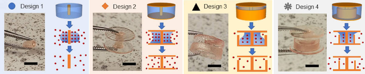
Finally, He and colleagues designed 8 mm-diameter tablets with different patterns of insoluble and soluble ink to create a range of release rates. They 3D printed four designs: an aspirin-loaded poly-ACMO tablet with a small insoluble core; a tablet capped top and bottom with insoluble surfaces; a capped and partially walled tablet with the wall at the outer radius; and a capped tablet with the partial wall nearer to the centre.

Printing tablets with different drug release behaviours

Measuring the release of poly-ACMO from tablets immersed in phosphate-buffered saline revealed that design 1 had the fastest release rate (4.07 mg/min). The insoluble barriers in design 2 reduced the release rate (to 2.17 mg/min), while the outer wall of design 3 reduced it further (to 0.98 mg/min). Design 4 showed an initial release comparable to design 2, then transitioned to a significantly lower release rate (0.70 mg/min) as the poly-ACMO front moved through the inner insoluble wall.

As the poly-ACMO dissolves, the tablets release aspirin with the same profiles: fast release for design 1, slow for designs 2 and 3, and a two-stage release profile for design 4. These findings demonstrate how co-printing soluble and insoluble structures can be used to programme drug release and introduce complexities, such as stepped drug release profiles, that can’t be achieved by traditional manufacturing methods.

The researchers note that the design flexibility of MM-IJ3DP holds potential for incorporating multiple pharmaceuticals in a single tablet, as well as manufacture of different tablet designs in a single production batch of 56 pills.

These unique capabilities could advance the field of personalized pharmaceuticals, the researchers say, enabling control of dose (by varying the quantity of drug-containing soluble material), release rate (governed by the surface area) and the time of release (controlled by the spatial distribution of the soluble component).

The team is now working to expand its database of formulations and design pills that maximize the technique’s capabilities. “We are currently investigating the use of AI technology to understand the drug release profiles of different 3D-printed pills,” He tells Physics World. “This approach will offer us a new toolset to help us design pills that meet the desired drug release performance specified by pharmacists for patients.”

Ursula Le Guin: the pioneering author we should thank for popularizing Schrödinger’s cat

The world’s most famous cat is everywhere. It appears on cartoons, T-shirts, board games, puzzle boxes and glow-in-the-dark coffee cups. There’s even a gin named after the celebrity animal. Boasting “lovely aromas of fresh mint and lemon zest”, with notes of basil, blueberries, cardamom and lemon-thyme – and “a strong backbone of juniper” – it’s yours for just £42.95 for 500 ml.

You know whom I’m talking about. But despite its current ubiquity, the fictitious animal only really entered wider public consciousness after the US science-fiction and fantasy writer Ursula K Le Guin published a short story called “Schrödinger’s cat” exactly 50 years ago. Le Guin, who died in 2018 at the age of 88, was a widely admired writer, who produced more than 20 novels and over 100 short stories.

Schrödinger originally invented the cat image as a gag. If true believers in quantum mechanics are right that the microworld’s uncertainties are dispelled only when we observe it, Schrödinger felt, this must also sometimes happen in the macroworld – and that’s ridiculous. Writing in a paper published in 1935 in the German-language journal Naturwissenschaften (23 807), he presented his famous cat-in-a-box image to show why such a notion is foolish.

For a while, few paid attention. According to an “Ngram” search of Google Books carried out by Steven French, a philosopher of science at the University of Leeds in the UK, there were no citations of the phrase “Schrödinger’s cat” in the literature for almost 20 years. As French describes in his 2023 book A Phenomenological Approach to Quantum Mechanics, the first reference appeared in a footnote to an essay by the philosopher Paul Feyerabend in the 1957 book Observation and Interpretation in the Philosophy of Physics edited by Stephan Körner.

The American philosopher and logician Hilary Putnam (1926–2016) first learned of Schrödinger’s image around 1960. “I always assumed the physics community was familiar with the idea,” Putnam later recalled, but he found few who were. In his 1965 paper “A philosopher looks at quantum mechanics” Putnam called it “absurd” to say that human observers determine what exists. But he was unable to refute the idea.

Invoking Schrödinger’s image, Putnam found that we are indeed unable to say “that the cat is either alive or dead, or for that matter that the cat is even a cat, as long as no-one is looking”. Putnam had another worry too. Quantum formalism required that if he looked at a quantum event, it would throw himself into superposition. Putnam concluded that “no satisfactory interpretation of quantum mechanics exists today”.

Enter Le Guin

It was to be another decade before the cat and its bizarre implications jumped into popular culture. In 1974 Le Guin published The Dispossessed (1974), an award-winning book about a physicist whose new, relativistic theory of time draws him into the politics of the pacifist-anarchist society in which he lived. According to Julie Phillips, who is writing a biography of Le Guin, she read up on relativity theory to make her character’s “theory of simultaneity” sound plausible.

“My best guess,” Phillips wrote in an e-mail to me, “is that she discovered Schrödinger’s cat while doing research for the novel.” Le Guin, it appears, seems to have read Putnam’s article in about 1972. “The Cat & the apparatus exist, & will be in State 0 or State 1, IF somebody looks,” Le Guin wrote in a note to herself. “But if he doesn’t look, we can’t say they’re in State 0, or State 1, or in fact exist at all.”

Le Guin was entranced by the implied uncertainties and appreciated the fantastic nature of Schrödinger’s image

Unlike Putnam, Le Guin was entranced by the implied uncertainties and appreciated the fantastic nature of Schrödinger’s image. “If we can say nothing about the definite values of micro-observables, when not measuring them, except that they exist, then their existence depends on our observation & measurement.”

In “Schrödinger’s cat”, which Le Guin finished in September 1972 but didn’t publish for another two years, an unnamed narrator senses that “things appear to be coming to some sort of climax”. A yellow cat appears. The narrator grieves but doesn’t know why. A musical note makes her want to cry but she doesn’t know for what, and thinks the cat knows but is unable to tell her. She then remembers Michelangelo’s painting The Last Judgment, of a man dragged down to hell who clamps a hand over one eye in horror but keeps the other eye open and clear. The doorbell rings and in walks Rover, a dog.

Black and white photo of a woman with short hair sat on a chair

Rover pulls a box out of his knapsack with a quantum-mechanical gadget that will either shoot or not shoot the cat once it gets inside and the lid is closed. Before we open the lid, Rover says, the cat is neither dead nor alive. “So it is beautifully demonstrated that if you desire certainty, any certainty, you must create it yourself.”

The narrator is not sure. Don’t we ourselves get “included in the system”; aren’t we still inside a yet bigger box? She’s reminded of the Greek legend of Pandora, who opens her box and lets out all its evil contents. She and Rover open the lid, but find the box empty.

The house roof flies off “just like the lid of a box” and “the unconscionable, inordinate light of the stars” shines down. The narrator finally identifies the note, whose tone is now much clearer once the stars are visible. The narrator wonders whether the cat knows what it was they lost.

Le Guin’s story was soon followed by other fictional and non-fictional treatments of quantum mechanics in which Schrödinger’s cat is a major figure. Examples include the Schrödinger’s Cat Trilogy (Robert Anton Wilson, 1979); Schrödinger's Baby: a Novel (H R McGregor, 1999); Schrödinger’s Ball (Adam Felber, 2006); Blueprints of the Afterlife (Ryan Budinot, 2012). There have also been a number of short stories including F Gwynplaine MacIntyre’s “Schrödinger's cat-sitter” from 2001.

The critical point

Phillips called Le Guin’s “Schrödinger’s cat” a “slight, playful story with an undercurrent of sorrow”, and warned me not to overthink it. “You could think of it as ‘a fantasy writer looks at quantum mechanics’,” she explained, adding that Le Guin wrote in her journal that fantasy as a genre and physics as a science are approaches to reality that reject common sense. “I think,” Phillips concluded, “she may have been playing around with her sense, at that moment, that physics was another way of expressing the fantastic.”

If so, Le Guin unerringly found the right image.

Copyright © 2026 by IOP Publishing Ltd and individual contributors