The pressure variations of a sound wave can make a gas bubble in a liquid periodically shrink and grow. At certain temperatures and pressures, the bubble may implode to generate a huge pulse of energy, which leads to the emission of photons. Many physicists believe that the gas inside the collapsing bubble is rapidly compressed and becomes so hot – typically 20 000 to 30 000 kelvin – that it becomes a plasma.
Most studies of sonoluminescence have focused on the effect of adjusting the pressure on the gas bubble – that is, using different frequencies and intensities of sound waves. But these experiments have been hampered by the narrow range of conditions under which sonoluminescence will take place.
According to Fink and co-workers, their technique overcomes these limitations. They filled a spherical glass cell with water and trapped an air bubble by focusing a 28 kHz standing wave onto it. This caused the bubble to oscillate in size between 5 and 50 micrometres in radius. Just as the bubble was about to collapse, the team switched on eight 700 kHz generators that were evenly spaced around the cell. These signals interfered constructively with the lower-frequency waves and made the bubble collapse more quickly, emitting nearly twice as much light as it did without them.
The team believes this method can be modified to make the bubble collapse even faster, which would lead to greater light intensities. This would allow physicists to study the relationship between pressure, light intensity and temperature in sonoluminescence in more detail.
Some physicists have suggested that a rapidly collapsing bubble could be used to compress nuclear fuel in order to initiate fusion reactions, although team member Jean-Louis Thomas emphasizes that this is some way off. Lasers are currently used to squeeze the fuel pellets in this technique, which is known as inertial confinement fusion.
‘The work done so far on sonoluminescence is largely academic and aimed at understanding the physics involved’, Thomas told PhysicsWeb. ‘We are still a long way from fusion but it doesn’t seem impossible’.
Black holes present obvious problems for would-be observers because they cannot, by definition, be seen with conventional telescopes – although before the end of the decade gravitational-wave detectors should be able to study collisions between black holes (see Physics World December 2001 pp10-11, print version). Until then astronomers can only infer the existence of a black hole from its gravitational influence on other matter, or from the X-rays emitted by gas and dust as they are dragged into the black hole. However, once this material passes through the “event horizon” that surrounds the black hole, we will never see it again – not even with X-ray specs.
Despite these observational problems, most physicists and astronomers believe that black holes do exist. Small black holes a few kilometres across are thought to form when stars weighing more than about two solar masses collapse under the weight of their own gravity, while supermassive black holes weighing millions of solar masses appear to be present at the centre of most galaxies. Moreover, some brave physicists have proposed ways to make black holes – or at least event horizons – in the laboratory (see Artificial black holes on the horizon and Analog models of general relativity).
The basic idea behind these “artificial black holes” is not to compress a large amount of mass into a small volume, but to reduce the speed of light in a moving medium to less than the speed of the medium and so create an event horizon. The parallels with real black holes are not exact but the experiments could shed new light on a variety of phenomena. The first challenge, however, is to get money for the research. One year on from a high-profile meeting on artificial black holes in London, for instance, the UK’s research councils have yet to put any real money behind these ideas.
Black holes are best described by the general theory of relativity. However, general relativity is a classical theory of gravity, and although its predictions have been verified in many experiments, a quantum theory of gravity remains one of the holy grails of physics. One of the first physicists to make real progress in this quest to reconcile general relativity and quantum mechanics was Stephen Hawking.
In 1974 Hawking calculated what would happen if a quantum fluctuation occurred near an event horizon. He concluded that the black hole would radiate, and that the amount of radiation would be inversely proportional to the mass of the black hole. However, black holes tend to be very heavy, so their output of Hawking radiation would be too low to detect experimentally. One intriguing exception could be much smaller primordial black holes created in the big bang: these should radiate observable amounts of gamma rays, but they have not been detected yet. This whole body of work – in which thermodynamic concepts such as temperature and entropy are also associated with the black hole – is Hawking’s major achievement in physics (see From the big bang to the eureka moment).
The detection of Hawking radiation is the ultimate goal of experiments on artificial black holes, although a lot of theoretical and experimental work has to be done first. The successful experiment is likely to involve a flowing Bose-Einstein condensate or a medium in which the speed of light can be reduced to zero (see Physics World February 2001 pp20-21, Black holes go supersonic (summary); September 2001 pp35-40, Taming light with cold atoms). After years of groundwork, physicists have recently made rapid progress in both these fields. Meanwhile, the recent observation of neutrons in discrete quantum states in a gravitational potential shows that quantum gravity effects can be seen in the laboratory (see Neutrons reveal quantum effects of gravity). All that is needed now is an act of faith.
Lubricants are essential in modern life. Car engines and gearboxes run smoothly thanks to sophisticated oils and greases, while computer hard disks rely on thin organic films to ensure that the “read/write” head can move reliably at high speeds across the recording medium. According to some analysts, however, the direct costs of friction and wear can account for nearly 10% of the gross national product (GNP) in many industrial nations. Moreover, they estimate that cost savings of up to 1% of the GNP could be achieved simply by using the right lubricant for the job.
Lubricants are remarkable fluids. During winter in Detroit, for example, the same car-engine oil has to operate reliably over temperatures ranging from -40 °C to above 250 °C – the temperature near the top piston ring. It also has to cope with pressures between 105 and 109 pascals, as well as contaminants including metal particles and soot. The final straw is that this fluid must deal reliably with these conditions every day for up to two years – the recommended time between oil changes, according to some vehicle manufacturers.
Surprisingly, one of the major driving forces behind the development of lubricants is the environment. Modern vehicles are required to emit far fewer pollutants than older cars and lorries. Indeed, the emissions from a typical modern vehicle are some 50 times lower than those manufactured in the 1960s.
Carbon dioxide is a natural by-product from the combustion of fuel and is among the most significant pollutants being targeted for reduction. Indeed, vehicles that have a high fuel consumption emit large amounts of carbon dioxide. However, the European Union is taking a strong lead in tackling this problem, and has indicated that the average amount of carbon dioxide emitted by every vehicle should be reduced from today’s average of 200 grammes per kilometre to less than 140 grammes per kilometre from 2008. This is roughly equivalent to improving the average fuel consumption from 33 to 47 miles per gallon. Such an increase would lead to big cuts in terms of carbon dioxide. In the UK alone – where there are roughly 20 million cars, each covering an average of 16 000 km every year – the total annual drop in CO2 would be about 19 million tonnes.
Clearly manufacturers are making a number of engineering changes to their vehicles to try to improve fuel economy. Less well known, however, is the fact that the fuel consumption can be significantly improved just by changing the lubricants. For example, it is possible to decrease the amount of fuel consumed by modern cars by up to 5% simply by switching from a typical multigrade oil to a “friction-modified” lubricant with a lower viscosity. This would lead to an annual CO2 drop of roughly 3 million tonnes in the UK. Remember that this figure is just for the UK and just for cars. Greater CO2 savings are clearly possible if optimized lubricants were also used in trucks and in other machinery.
What is a lubricant?
Car lubricants play four major roles – they control friction and wear in the engine, they protect the engine from rusting, they cool the pistons, and they protect the engine oil stored in the sump from combustion gases.
Some 75%-95% of a typical engine lubricant is made up of a base oil – a mineral oil that has come directly from a refinery. These base oils can naturally contain straight or branched chains of hydrocarbons, hydrocarbon molecules with aromatic rings attached, or these chains can be produced by further chemical reactions of the base oils.
The remainder of the lubricant comprises a variety of additives, which are used to improve performance. Typically these include anti-wear additives, corrosion inhibitors, antioxidants, detergents, dispersants, antifoam additives, and large polymer molecules known as viscosity modifiers, which are added to improve the viscosity variation of the lubricant with temperature.
Indeed, the viscosity is the most significant physical property of a lubricant. The way in which it varies with temperature, shear rate and pressure determines to a great extent how the lubricant performs in an engine. But the chemistry of the lubricant is also important: it must be resistant to oxidation and it must be able to “lay down” a protective film to combat wear and tear where metallic contact is inevitable.
The behaviour of an oil film trapped between two moving surfaces is quantified by the dynamic viscosity, which is measured in millipascal seconds (mPa s). More accurately, the dynamic viscosity relates the shear stress, the shearing force acting on the oil per unit area, and the shear rate, the difference in velocity between the two surfaces divided by their separation. However, it is often more convenient to measure a quantity known as the kinematic viscosity, which is the dynamic viscosity divided by the fluid density and is measured in mm2 s-1 or centiStokes (cSt).
Lubricants fall into two broad categories – monograde and multigrade – depending on whether their viscosity changes significantly with temperature or not. A more detailed classification system has been devised by the Society of Automotive Engineers (SAE) (see table). One common lubricant is described according to this scheme as an SAE-10W/30 multigrade. The first number (10W) refers to the dynamic viscosity measured at low temperatures, while the second (30) describes the kinematic viscosity at 100 °C. Lower numbers describe runnier lubricants – the viscosity of an SAE-5W/30 multigrade, for example, is five times lower than that of SAE-20W/50 at -20 °C. Roughly speaking, the energy lost due to friction varies with the square root of the viscosity: at -20 °C the friction losses of the low-viscosity oil will be approximately half those of the thicker oil, allowing the engine to start more easily.
The viscosity grade of a multigrade oil is different at high and low temperatures due to additives known as viscosity modifiers. For example, SAE-10W/30 has a similar viscosity to the monograde lubricant SAE-30 at 100 °C. At lower temperatures, however, SAE-10W/30 is much thinner than the monograde oil. This means that the multigrade oil provides protection at high temperatures and is runny enough at low temperatures to enable engines to start easily in most European countries. In contrast, the thick monograde oil would simply be unsuitable in winter.
Lubricants make the grade
Viscosity grade
Kinematic viscosity at 40 °C (cSt)
Kinematic viscosity at 100 °C (cSt)
Dynamic viscosity at -15 °C (mPa s)
SAE-30
91.3
10.8
3950
SAE-20W/50
144.8
17.8
5870
SAE-15W/40
114.3
14.9
2940
SAE-10W/30
72.3
10.8
1900
SAE-5W/30
57.4
9.9
1090
SAE-0W/20
44.4
8.3
690
The typical viscosities of common lubricants as graded according to the Society of Automotive Engineers’ J300 classification. A multigrade oil described as SAE-15W/40, for example, is a grade 15 at low temperatures and a grade 40 at high temperatures. For an oil to be a grade 15, the dynamic viscosity at -15 °C has to be less than 3500 mPa s, while the kinematic viscosity of a grade 40 oil must be between 12.5 and 16.3 cSt at 100 °C.
Well-oiled components
In a typical gasoline internal-combustion engine, fuel enters the combustion chamber when an inlet valve opens. This valve then closes and the piston moves upwards, compressing the fuel-air mixture. When the piston reaches its highest position, the spark plug is activated and combustion occurs, pushing the piston back downwards. The translational motion of the piston is then converted into rotational motion via the connecting rod and the crankshaft bearings.
For an engine to work effectively, the contacts between the cams (which push the valves controlling the inlet and outlet to the combustion chamber) and the tappets (which operate the valves) must be adequately lubricated so that the components do not wear excessively. A complete oil film must also be formed between the piston rings and the piston liner to prevent wear, to seal the combustion-chamber gases from the rest of the engine, and to minimize friction losses. Finally, a thick film of oil must cover the engine bearings so that the metal surfaces in the bearing do not come into contact.
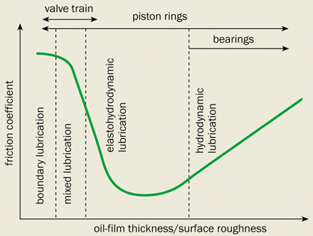
1 Zone-in on lubrication The variation of the friction coefficient as a function of oil-film thickness divided by surface roughness. Four distinct lubrication regions are observed. Some components, such as the engine bearings, operate solely in the hydrodynamic-lubrication region, while others undergo two or more different types of lubrication. (Courtesy: IOP Publishing)
A typical engine oil is carefully formulated to protect the valve train, the bearings and the piston assembly, despite the different lubrication requirements of these components. In fact, the thickness of the oil determines its coefficient of friction and defines four distinct regions of lubrication (figure 1).
Engine bearings and the piston mostly operate in the “hydrodynamic lubrication” region, where a thick film separates the moving metal surfaces so that there is no chance of them coming into contact. When the pistons are momentarily stationary, however, the layer of oil covering them can be similar in thickness to the surface roughness of the components. In this “mixed lubrication” region, the metal surfaces intermittently come into direct contact. If the thickness of the oil film is much smaller than the surface roughness then the metal surfaces rub together repeatedly – this is known as “boundary lubrication”. Contact between the cams and the tappets in the valve train span the mixed and boundary regions.
The final type of lubrication – elastohydrodynamic lubrication – occurs under high loads and is commonly encountered with hydrocarbon-based oils. Here the pressure developed in the lubricant is sufficiently high to elastically deform the metal surfaces either side of the oil film. This happens because the viscosity of these fluids increases significantly as the pressure rises. The valves and the piston rings occasionally operate in this region.
Lubricants are also used in other important components in a vehicle, including the gearbox. This is a challenging environment where pressures routinely exceed 109 Pa and the gears operate in the elastohydrodynamic-lubrication regime. Moreover, in many cars the gear lubricant is filled once and then never replaced during the vehicle’s lifetime. Even so, researchers at Torotrak in Leyland, UK, are currently developing novel transmission systems that are effectively gearboxes with an infinite range of gear ratios. These continuously variable transmissions are designed to ultimately improve fuel efficiency and they require lubricants that have special properties, such as very high friction coefficients, which our group at Shell’s Cheshire Innovation Park is developing in collaboration with Torotrak.
Greases are also commonly used to lubricate the constant-velocity joints that connect the axles to the drive wheel while allowing the suspension to move up and down. These joints are critical components in many current models of four-wheel-drive and sports-utility vehicles and they therefore require high-performance greases.
Measurements smooth the way
Most engine manufacturers design their components to operate with oils and greases within a certain viscosity range. It is therefore important to be able to measure the properties of lubricants accurately.
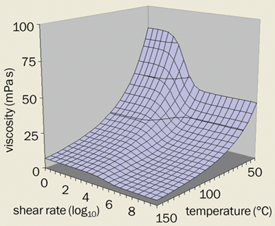
2 Variations in viscosity The viscosity of an SAE-10W/50 engine lubricant as a function of shear rate and temperature. In general, the oil becomes thicker at low temperatures and when the shear rate is small. The viscosity decreases at high shear rates due to the addition of viscosity modifiers, long hydrocarbon molecules that align in the direction of the shearing force. (Courtesy: IOP Publishing)
The kinematic viscosity of oil is usually determined under low shear rates, simply by measuring the time the meniscus takes to flow vertically downwards between two marks on a capillary tube. Different diameter capillary tubes are used for thinner or thicker oils.
Meanwhile, the dynamic viscosity is usually measured under the high shear conditions – and sometimes the high temperatures – typically found in bearings and other critical contacts in engines. These measurements are carried out by instruments in which a thin film of oil is trapped between two surfaces moving relative to each other. For example, in a “rotating cylinder viscometer”, the dynamic viscosity is estimated from the shear torque produced on a stationary inner cylinder by a revolving outer one. Another instrument that is used for measuring very small quantities of lubricant, in particular, comprises a conical surface rotating against a flat plate coated in oil.
These measurements can also tell us something about how the viscosity varies with shear rate. Our group at Shell and others, including Jagadish Sorab at Ford, have fitted such data to realistic equations that describe how the viscosity varies with both temperature and shear rate (figure 2). We have found, for example, that the viscosity of a typical engine lubricant decreases at high shear rates. The reason is that the large polymer molecules used as viscosity modifiers line up in the direction of the shear force at high shear rates. This alignment reduces the “thickening” effect that these polymers have when they are randomly aligned.
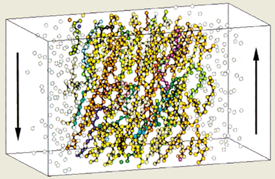
3 Go with the flow Non-equilibrium molecular-dynamics simulations confirm that the hexadecane molecules in this model lubricant temporarily align in a shear field. (Courtesy: IOP Publishing)
Indeed, non-equilibrium molecular-dynamics simulations of model lubricants carried out by physicists at Shell in the early 1990s clearly show how the molecules line up when a high shear rate is applied to the fluid (figure 3). The effect, however, is temporary – the viscosity returns to its previous value when the shear rate is reduced.
Crucially for automotive applications, these types of experiments have also revealed how the viscosity of a lubricant varies with pressure. For example, the viscosity of a typical lubricant at 500 MPa can be between 10,000 and 100,000 times higher than that at atmospheric pressure. Roughly speaking, the viscosity increases exponentially as the pressure increases. This exponential variation is known as Barus’s law and is valid at pressures up to a few hundred megapascals. At very high pressures (2-4 GPa), however, this simple relationship tends to overestimate the increase in viscosity. Instead the lubricant becomes glass-like and behaves more like a solid than a liquid, deforming the metal surfaces on either side of the lubricant elastically – this is the elastohydrodynamic-lubrication regime.
Elastic effects
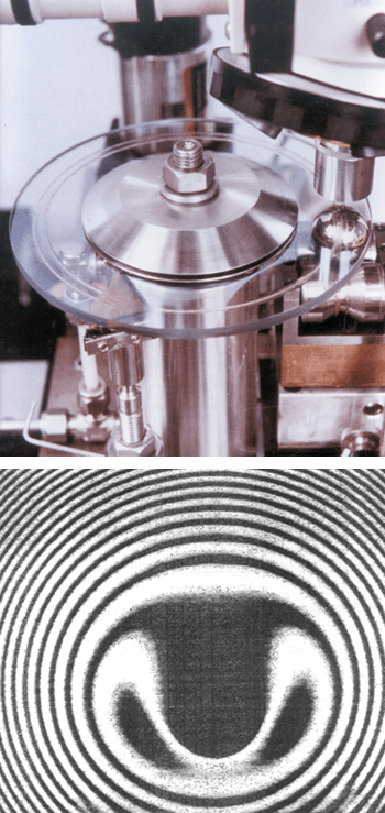
4 Fringes benefit lubricants Top: A ball-on-plate rheometer used to measure the properties of lubricants in the elastohydrodynamic region. A steel ball is pressed against a transparent rotating disk made of glass or sapphire. As the disk rotates, the thickness of the oil film between the two components is measured by shining light through the transparent disk and monitoring the interference fringes. Bottom: This characteristic pattern of interference fringes shows that the thickness of the oil film at the centre of the contact is approximately constant, while the film at the edges is thicker.
Other optical and mechanical techniques have been developed to investigate the behaviour of oils and greases in the elastohydrodynamic region. One of the most common instruments used for this purpose is the so-called ball-on-plate rheometer, which was first used extensively by Hugh Spikes’ group at Imperial College in London in the 1980s. Essentially the instrument consists of a steel ball that is pressed against a transparent rotating disk made of glass or sapphire. As the disk rotates, the thickness of the oil film between the two components is measured by shining light through the transparent disk and monitoring the resulting interference fringes (figure 4, top).
When the ball is pressed lightly against the disk, the surface remains unaltered and a series of concentric circles is observed. However, if the ball is pressed hard against the disk, then the plate deforms elastically, as shown by the characteristic horseshoe-shaped interference pattern (figure 4, bottom). This shape indicates that the thickness of the oil film at the centre point of the contact is approximately constant, while the increase in the number of fringes outside the central region demonstrates that the film is thicker at the edges. In this elastohydrodynamic region, the flat central region behaves in a similar way to a ball of Plasticine pressed against a flat surface, with the difference that the surfaces return to their original shape when the pressure is removed.
Elastohydrodynamic lubrication occurs in gears, valve trains and in the “rolling-element bearings” found in wheel hubs, which have to cope with large radial and thrust loads with minimum friction. The ball-on-plate rheometer is therefore ideal for evaluating the performance of lubricants under the realistic conditions found in many machine components.
Other methods for measuring the viscosity of lubricants under high pressures include the “falling ball” experiments pioneered by Bo Jacobson, now at Lund University in Sweden, and co-workers in 1985. In these experiments, a steel ball is dropped either vertically, or more commonly at an angle, onto a plate smeared with a drop of oil or grease. Pressures of up to 7.5 GPa can be created in the lubricant film in this way. And the coefficient of friction can be determined from either the motion of the ball after contact, or from force transducers on the surface. Different lubricants have different friction coefficients because of the way that the viscosity varies with temperature, shear rate and pressure.
Finally, it is worth mentioning that many lubricants also exhibit some elastic effects – in other words their behaviour cannot be fully explained just by assuming that they are purely viscous fluids. Grease, for example, is viscoelastic: under certain conditions it behaves as a viscous fluid – for instance when it flows freely in a pipe under an applied pressure; on other occasions, it behaves like a solid, for example prior to flowing. Most other commercially available lubricants also exhibit viscoelastic behaviour, albeit to a lesser extent.
Rheometers can also be used to measure viscoelastic properties as well as viscosities. However, little is known about how these attributes vary with temperature, pressure and shear rate because these measurements are difficult to make for commercial lubricants that have weak viscoelasticity. However, several researchers – including Brian Williamson at Shell and Ken Walters at the University of Wales in Aberystwyth – currently speculate that viscoelastic lubricants form thicker oil films in engine bearings under extreme conditions than less elastic fluids.
Grease-lightning simulations
With the increased computer capacity that has become available over the last decade, it is now possible to accurately model the performance of lubricants in engines, gearboxes and other components. For example, if we know the minimum thickness of the oil film, we can predict the durability of the component and the power loss due to friction. This capability can help researchers who are designing new lubricants to predict how a machine’s performance is related to lubricant viscosity, and how it will be affected by temperature, shear rate and pressure.
The theory of elastohydrodynamic lubrication was first developed by Duncan Dowson at Leeds University, and others, in the 1950s, when computer simulations were not possible. In elastohydrodynamic lubrication both the fluid equations and the elastic deformation of the surfaces have to be modelled, and these complicated simulations can now be performed on modern computers relatively quickly. Meanwhile, hydrodynamic lubrication in plain bearings and piston rings can be analysed in seconds. Modelling mixed and boundary lubrication is more difficult since we require a detailed understanding of the roughness of the surfaces as well as of the lubricant properties. In general, the output of the models is the minimum thickness of the oil film and the losses due to friction.
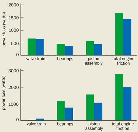
5 Where’s the rub? Computer models are now being used to predict the power lost due to friction in each engine component. The results can also be combined to estimate the total losses in this 2 litre European gasoline engine operating at 100 °C (top) and 40 °C (bottom), and under medium load. Physicists and engineers can study the effects of two different lubricants, a friction modified SAE-5W/30 (blue) and a standard SAE-15W/40 grade (green) at different temperatures. The losses are much higher at low temperature due to the losses that occur in the hydrodynamically lubricated components, such as the bearings and the piston assembly. On the other hand, power losses in the valve train decrease with the lower temperatures. This 40% increase in friction for the thicker oil corresponds to an increase in fuel consumption of about 12%. Changing to a lower-viscosity-grade lubricant would lead to a decrease in engine friction that could correspond to an improvement of 4% in fuel consumption. Fuel-economy benefits, however, are difficult to demonstrate in practice because many factors, such as weather conditions, engine conditions and driver behaviour can have a much more significant effect on fuel consumption than the lubricant. (Courtesy: IOP Publishing)
Many groups have accurately estimated the minimum oil-film thickness in an elastohydrodynamic contact. However, estimating the friction coefficient has proved much more problematic due to the large variation of viscosity with pressure, which is not always accurately known. Recently, Laurence Scales at Shell has shown that it is worth investing the effort to find accurate relationships between viscosity, temperature, pressure and shear rate because they allow both the minimum oil-film thickness and the friction coefficient to be estimated. To do this, however, requires at least eight parameters to characterize the lubricant.
But by combining models for the plain bearings, the piston assembly and the valve train, researchers have found that they can model the lubrication conditions in a complete internal combustion engine. Since the bearings and piston rings are lubricated predominantly in the hydrodynamic regime, a lubricant with a lower viscosity should lead to a thinner oil film and thus lower friction. However, the valve train operates in the mixed-boundary lubrication regime, which means that lower friction can only be obtained with thicker lubricants. Engine-friction models enable us to study the trade-off between viscosity and friction, and therefore select the optimum lubricant to improve a vehicle’s fuel economy (figure 5).
Future challenges
There are many challenges in developing the lubricants of the future. Cars are becoming more powerful, drivers would like to change the engine oil less frequently, and manufacturers want to reduce the losses due to friction even further. In order to develop lubricants that satisfy these demands, physicists and engineers have to understand the performance of the lubricant in more detail.
First, we need to fully understand the role that the elastic properties of lubricants play under extreme conditions. To do this we will need to measure the viscoelastic properties of lubricants at different temperatures, pressures and shear rates, and develop a suitable model. Our current models are based on the Reynolds’ equation, which assumes that the oil film is of the order of a few microns thick and that the components are a few millimetres across. A more serious shortcoming of the Reynolds’ equation is that it assumes that elastic effects are not important.
The second major challenge is to incorporate chemistry into physical models. After all, lubricants change chemically during their time in an engine. Simply speaking, a fresh lubricant is like a pure hydrocarbon. Over time, however, it oxidizes and chemically degrades to form alcohols, ketones, aldehydes, acids and esters. These chemical changes can lead to an increase in viscosity. The present author is currently developing a chemical model that also simulates the reactions in an engine, in collaboration with Martin Priest at Leeds University and John Lindsey-Smith at York University, both in the UK. The aim is to determine the chemical composition of the lubricant in the sump at any instant and, in principle, the increase in viscosity, which would then feed into the physical models discussed earlier. However, this still leaves the challenge of understanding the physics and chemistry in the boundary-lubrication region.
Safeguarding the environment
Physicists are playing an increasing role in addressing the environmental problems of pollution and global warming, as well as in understanding natural climate phenomena such as El Niño. Ever-more-sophisticated experiments are revealing that lubricants are a rich source of physics, and physicists are quick to use these findings to design environmentally friendly lubricants that will help to reduce our impact on the planet. The progress that is being made in lubricant research today will undoubtedly play a part in safeguarding the natural environment for many generations to come.
To what extent can drama provide an insight into the scientific enterprise? And to what extent can theatre be used as a vehicle for exploring the history of science? These questions are more than just of esoteric interest, following the huge success of historical plays like Copenhagen, which examines the war-time meeting between Bohr and Heisenberg, and others based on episodes or figures from history, such as Breaking the Code and QED.
Playwrights have been using the stuff of history from earliest times, and historical drama, in its many forms and variations, is a well established genre in Western theatrical tradition. Yet the two – history and drama – do not necessarily have compatible goals. They also differ in how they try to achieve these goals. As the Italian dramatist Luigi Pirandello playfully noted, truth doesn’t have to be plausible, but fiction does.
Thus, the historian of science must at times accept the chaotic and the contingent, the randomness and even the apparent meaninglessness of events and actions. The playwright, however, must work with a structured logic grounded in dramatic conventions. Indeed, playwrights have been known to reject historical truths because they appear so implausible: on stage the actual events might seem too contrived or the villains too melodramatic or too passive. Instead, the constructed drama presents an artifact more plausible, seemingly truer, than the actual historical record.
But how far dare the dramatist deviate from that record? And, of course, whose authoritative record are we referring to when treating a controversial subject?
Drama and deeper truths
Drama on stage is much more seductive as a representation of history than scholarly texts. Thus even non-realistic depictions that do not purport to represent faithfully events and persons still tend to make the audience feel that they have experienced history. And even when the audience is well aware that the factual content of a history-based play is false, they may still find the play engrossing, urgent and in touch with some deeper truth.
It is often argued that playwrights must sometimes depart from historical detail in order to provide accurate and engaging portrayals of the underlying historical forces. The problem is that, on closer inspection, such plays depict and probe not the social relations or political processes at the time of the subject, but those of the dramatist instead. Classical historical plays – be it the works of Shakespeare, Schiller, Strindberg or Brecht – seem to address the political realities of their own times, rather than those of the previous eras in which they are set. True, historians also write with the present and future in mind, but they necessarily must interpret and seek understanding from within the relevant historical context derived from that particular time and place.
So why must dramatists use people and events from history when their purpose is to illuminate an argument or to provoke discussion? The answer can be seen in Friedrich Dürrenmatt’s 1962 play The Physicists, in which the author frees himself from actual facts and personalities in order to mould a drama that playfully, but forcefully, raises questions about ethical responsibility for research. In the play, Dürrenmatt creates three fictional physicists in an asylum, who claim to be Newton, Einstein and King Solomon. But are they mad, or simply acting mad to ensure that the nuclear secrets they have uncovered will remain out of the hands of those who might use them for evil? The play, which became a fixture in post-war theatre, engages the audience intellectually and emotionally, without referring to actual historical episodes.
Drama and real history
But what if the playwright begins not with a fictional plot or an imaginary set of characters, but with a real historical episode? What if the stuff of history appears so compelling, so electrifying, that the dramatist decides to shape it, mould it and pound it into a workable dramatic structure?
Of course, for professional historians of science, that which normally holds our interest may not be the stuff of drama at all. But many of our concerns are certainly of more than academic interest. Drama may well reside, for example, in scientists’ social, moral and professional dilemmas, such as their struggle for recognition, for resources, for arriving at new findings, and for gaining acceptance of these. If theatre is chosen as the vehicle for exploring such episodes, we must accept a basic truth: theatre cannot readily depict narrative history unfolding over time and ought not to try.
Drama can stimulate thought and raise questions. No medium can better convey the immediacy of emotions – and science, after all, entails not only cold logic but also cauldrons of hot passion. Theatrical convention can be used to explore the complexity of a scientist’s emotional, intellectual and moral make-up. Although never a substitute for history, a play based on history that is crafted by a skilled and intellectually able dramatist can open windows onto aspects of science that can prod audiences to reflect on or read further about. The pay-off is the degree to which particular scientific events and the personalities connected with these are thereby allowed to enter our cultural heritage and popular imagination – rather than remaining the property of academic historians and scientists.
Consider a play such as Michael Frayn’s Copenhagen. Although primarily concerned with the slippery nature of historical reconstruction and the epistemological problem of what we actually can know of other people’s – and our own – motives, it has clearly brought significant chapters in the history of modern physics to the attention of many non-specialists. In exploring the events in 1941 when Werner Heisenberg visited Niels Bohr in Nazi-occupied Denmark, Frayn chooses a fictive situation for the drama: the historical characters return from the dead and try to make sense of what did or did not happen.
Frayn provides a wonderful display of intellectual and emotional fireworks. Although he makes no claim for the play to be actual history, he also notes (in the preface) his indebtedness to a number of historians, who themselves disagree in interpreting what actually took place at that legendary 1941 meeting.
But regardless of the playwright’s intentions and even extreme care in creating his characters, audiences may leave the theatre with a wide range of impressions. In the case of the London production of Copenhagen on the evening that I attended, members of the audience with whom I spoke came away believing Bohr to be no better morally than Heisenberg; perhaps even less sympathetic. I am not sure, however, that this was the playwright’s intention. Without second-guessing Frayn’s own meaning and without wanting to judge the ability of an audience on a Friday evening to grasp nuance, I felt uncomfortable.
How malleable is history?
Perhaps I am being over-sensitive. Nevertheless, in a TV film for which I wrote the screenplay, a German scientist was to appear in a Wehrmacht uniform as a member of the armed forces. The director, however, dressed him in the uniform of the SS. This shamed a man who was still alive in the memory of his colleagues and family. True, accidents and mistakes do occur in film and theatre productions. The problem is that small adjustments in interpretation of the dramatic text by a director or performer for the sake of artistic effect can result in a deviation from what might be considered a reasonable portrayal of a person from history. And given that theatre audiences have been known to down more than a few drinks during the interval, should playwrights avoid complexity in plot and thought in the second half? Needless to say, the writer who obsesses over such angst-inducing concerns will not get much down on paper.
I have for some time been sketching ideas for plays based on my own historical research. Some of the scientists involved lived not too long ago. But when dramatizing the history of science, we are on terrain that is generally foreign to traditions in historical drama. Playwrights usually tend to choose historical characters who have already achieved legendary status: kings, queens, statesmen and others who are already public property. Audiences can then appreciate how the dramatist has interpreted or altered received history to make a point of contemporary importance. Few scientists, however, have achieved such status. Most scientists are not only not legendary but are hardly known to the public. Even practising scientists have little insight into any but the most well known researchers of times past.
When a playwright breathes life into a name from history and creates a seemingly real person who is as new for the audience as any fictional character, there should be some sense of responsibility for how that person is portrayed. Some directors and playwrights might say that the artist is only responsible to art: nobody takes theatre to be more than theatre. Historical drama, they might argue, has its own conventions and traditions; it does not purport to be history.
This may well be the case, but is it simply a matter of prudishness that brings me back to the question: just how malleable is historical scholarship in the forge of artistic imagination before intellectual and moral integrity snaps?
* This article is based on comments given by the author at the symposium Copenhagen and Beyond: Drama Meets History of Science organized by the Niels Bohr Archive in Copenhagen on 22-23 September 2001.
Books by the author
Appropriating the Weather: Vilhelm Bjerknes and the Construction of a Modern Meteorology: Amazon UK/Amazon US
The Politics of Excellence: Behind the Nobel Prize in Science: Amazon UK/Amazon US
Stephen Hawking is the most famous physicist in the world. Indeed, the sales of Hawking’s books and his appearances on The Simpsons and Star Trek have tended to overshadow his scientific achievements. But that was not the case in Cambridge last month when Hawking’s contributions to physics and cosmology were celebrated at a week-long conference to mark his 60th birthday. After graduating from what he told the meeting was “the very easy physics degree at Oxford”, in 1962 Hawking moved to Cambridge where he hoped to work on a PhD under Fred Hoyle. However, Hoyle already had too many students and Hawking reluctantly switched to the tutorship of Dennis Sciama, who had been one of Paul Dirac’s few graduate students.
During his PhD, Hawking was diagnosed as having motor neurone disease and was only given a few years to live. Instead he went on to become one of the leading theoretical physicists of his generation and, in 1979, was appointed to the Lucasian chair in mathematics at Cambridge – the same professorship that had been held by Newton and Dirac.
Looking back and forward
“We organized the meeting to look back on the immense contribution that Stephen has made to many areas of gravitational physics and cosmology,” said Gary Gibbons, one of Hawking’s colleagues at Cambridge. “We also wanted to look forward to what the future might hold for theoretical physics and cosmology, with special reference to the areas that Stephen has been most interested and most active in.” But Hawking almost did not make it to the conference – he crashed his wheelchair into a wall a few days after Christmas and had to have a metal plate inserted in his femur.
Hawking made his name with a series of papers in the 1960s on singularities in cosmology. Building on work by Roger Penrose, he showed that Einstein’s general theory of relativity implied that space and time would have a beginning in the big bang and would end in a singularity. “It was a glorious feeling, having a whole field virtually to ourselves,” Hawking told the meeting. “How unlike particle physics, where people were falling over themselves to latch onto the latest idea. They still are.” Hawking then switched his attention to black holes – regions of space where gravity is so strong that nothing can escape. He was also one of the first physicists to make progress in combining general relativity – the classical theory of gravity – and quantum mechanics.
First he showed that when two black holes collide and merge, the area of the “event horizon” around the resulting black hole is greater than the sum of the two original areas. This led Hawking and co-workers* to link the area of the event horizon, A, with the entropy of a black hole, S. Hawking told the meeting that he wants this simple equation (S = Akc3/4hG) to be on his tombstone.
Hawking then went on to predict that black holes have a temperature and are not, therefore, completely black. In simple terms, what is now known as Hawking radiation is produced when quantum fluctuations give rise to pairs of short-lived virtual particles near the event horizon. The gravity of the black hole pulls one of the particles from each pair into the black hole, while the other escapes. From a distance it appears as if the black hole is radiating. This effect was symbolized by the conference mug, which changes from black to white to reveal the equation for the Hawking temperature when it is filled with hot tea or coffee.
One speaker showed the meeting a list of Hawking’s papers in the SPIRES database at the Stanford Linear Accelerator Center. Six of Hawking’s papers have qualified for “renowned” status, having been cited more than 500 times by other papers in the database. The paper on Hawking radiation had the most citations, followed by a paper with Jim Hartle on the initial wavefunction of the universe, and a paper on the inflationary theory of the early universe.
The struggle to develop a quantum theory of gravity and to unify the four fundamental forces of nature was an overarching theme at the conference. Most theorists believe that the best approach is so-called M-theory, in which the fundamental particles are actually vibrations in tiny strings in a 11-dimensional space-time. So far theorists know that M-theory embraces a classical theory known as 11-dimensional supergravity and all five of the superstring theories that were previously candidates for a unified theory. However, they do not yet know how to apply M-theory to the real universe.
Close to the edge
While the meeting was dominated by black holes, M-theory and quantum cosmology, there were lighter moments. A Marilyn Monroe lookalike sang “I want to be loved by you” to Hawking at his birthday party, and The Edge – guitarist with the rock band U2 – attended the final day.
Hawking also confirmed himself as the master of the soundbite. “It has been a glorious time to be alive and doing research in theoretical physics, and I’m happy if I have made a small contribution,” he said in remarks that were widely reported in the media the following day. “There’s nothing like the eureka moment of discovering something that no one knew before. I won’t compare it to sex, but it lasts longer.”
The following correction appeared in the April 2002 issue of Physics World (page 20):
The articles “From the big bang to the eureka moment” and “Black holes and beyond” (February p9 and p13) should have made clear the role played by Jacob Bekenstein in the development of the concept of black hole entropy and the formulae for it and the temperature of a black hole (see, for example, Lettere al Nuovo Cimento4 737 (1972) and Phys. Rev. D 7 2333 (1973)).
The momentous complexity of modern physics is often seen as a stumbling block whenever one is asked to explain to the wider public – or to new students – how beautiful all of it is, and how unique and compelling are the logical deductions that have led to our present understanding. Many theoretical physicists have tried to do exactly this: to convey to the public not only what their findings are, but also why they think these findings are startling, and how these appear to reveal some deep underlying unity in the laws of physics.
Those who take on this task must act like a musician who wishes to enchant his audience with the beauty of a piece of music that is extremely difficult to play. If his skills are not quite up to the task, the musician might omit some of the most difficult notes or phrases, but in so doing he is sure to mutilate the composer’s masterpiece – even if the audience in question might not notice anything amiss. The truly professional musician, of course, manages to play even the most difficult parts in such a way that the message comes across in full, and the listener only hears the beauty of it, without even noticing that the piece is hard.
Modern physicists are in a worse position than musicians. Most physical theories have to be drastically reformulated before one can even think of making them digestible for non-experts. In Hidden Unity in Nature’s Laws, John Taylor attempts to do just this. However, he has chosen his musical instruments carefully. Galileo’s findings and Newton’s laws are usually taught using modern terminology, as this will surely carry us further when we arrive at the intricate structures of contemporary physics. Taylor, in contrast, exploits the fact that purely geometrical arguments can be pictured rather vividly.
Such an approach certainly works for the “old” physics, but can one use geometry to describe Maxwell’s laws of electromagnetism, quantum mechanics or the interactions between subatomic particles? What does gauge invariance mean in geometrical terms? What is the geometry of Heisenberg’s uncertainty relations? To explain all of this using practically no formulae at all should be considered an art form. Indeed, geometry can be used to argue that the number of particles inside the heaviest white dwarfs is related to the number of particles inside the heaviest allowable planets as 137 x (137)1/2, give or take a coefficient of order one.
What makes this book attractive for the professional physicist – as the well as the layreader – is its rich array of historical facts, references and descriptions of the achievements of past researchers, some of whom are not widely known. It is good to show respect for these scientists, given how much they had to struggle to discover those feats that nowadays are so commonplace to us.
It was not obvious at all, for example, that the Sun – not the Earth – had to be at the centre of the planetary system, and that the planets do not move in circles at fixed distances from us. It is delightful to read about the heated discussions on the nature of light between Newton and Huygens.
A problem with this approach is that the reader does expect the historical information to be accurate. For example, Taylor refers to Karl Schwarzschild as “at least one person who [already in 1916] quickly understood Einstein’s theory [of general relativity]”, and then continues to describe the co-ordinates used in our modern notation as the ones invented by Schwarzschild. Although it is universally accepted that Schwarzschild discovered the black-hole solution, if you read his paper you find out that, yes, he did understand the equations, but no, not the theory. Indeed, he made a big point of using “correct co-ordinates”, that is the ones where the black-hole horizon is imaged at the origin. This requirement would, he thought, have physically observable consequences. Naturally, Schwarzschild did not immediately understand the peculiar physics of the horizon.
Elsewhere, we read about the famous measurements of the speed of light carried out by the 17th-century Danish astronomer Ole Rømer. However, the values the author gives for the distance between the Sun and the Earth and for the time that light takes to travel this distance are incorrect by a factor of two. I think that astronomers of the time knew these numbers better than that even then.
A few other minor criticisms also spring to mind. Both from a historical and a conceptual point of view, it is a bit odd to discuss quantum chromodynamics and its basis in the Yang-Mills equations before the electroweak theory. Peter Higgs, meanwhile, did not introduce the four-scalar field components in the Standard Model of particle physics; he introduced the general principle now called the Higgs principle only for the U(1) case. Good accounts of the history of these developments can, however, be found elsewhere – both at the professional level in the proceedings of several recent Erice summer schools, and in a very journalistic style by Robert Crease and Charles Mann in their delightful book The Second Creation (1986 Macmillan).
I also found many of the figures in Taylor’s book to be poor and rather too sketchy, as if they were redrawn by someone who had little understanding of what they were supposed to convey. I like my parabolas to look like parabolas and my sine curves to look like sine curves.
But these are minor points. What makes this book extremely valuable is that the author has succeeded in adhering to his geometric approach throughout, starting with Galileo and ending with Ed Witten and Stephen Hawking. He explains their discoveries in physics in a lucid way using hardly any formulae, while avoiding over-simplifications and lacing the narrative with fascinating historical details.
Bobsledding is notoriously expensive – it typically costs $15-30m to create a world-class track and over $25 000 to design and test a competitive sled. Moreover, bobsled teams in the US and Asia can run up large travel bills since all but four of the tracks certified by the International Bobsledding and Tobogganing Federation (FIBT) for world-cup competition are in Europe.
These financial incentives have motivated the use of simulators, similar to those in commercial aviation, to teach the intricacies of bobsled driving. At the University of California at Davis, our group has developed such a simulator and installed two of them permanently at the US Bobsled Federation facilities in Lake Placid and Salt Lake City. The simulators allow athletes to train all year round for the world-cup circuit and the Olympic games (see A Kelly and M Hubbard 2000 Sports Engineering3 13).
Although existing one-dimensional studies of bobsled dynamics and sled performance are useful, to design a simulator we need to fully characterize the surface of the track and the motion of the sled in three dimensions. We base our mathematical models of various bobsled-track surfaces on measurements of the permanent concrete or stone foundations, which are covered with several centimetres of ice. Indeed, the surface in our models is accurate to about 4 mm and is more precisely known than the surface of the ice itself.
The track surface is then incorporated into three differential equations that describe the motion of a body that slides along the track with one rotational and two translational degrees of freedom. These equations also contain various vehicle parameters, such as the mass of the sled, its moments of inertia, aerodynamic drag and lift coefficients, and the coefficients of friction for the steel runners on the ice. We also need to know exactly how the driver steers the sled in his or her attempt to control the vehicle.
Steering to victory
Bobsled events are frequently finely contested. At the 1998 winter Olympics in Japan, for example, Great Britain and France tied for the bronze medal having taken exactly the same time to complete four runs, while the US team came in fourth just 0.02 seconds behind.
The driver’s job is to manoeuvre the sled to minimize the time it takes to complete the course. But controlling the sled is an extremely delicate task because only the front runners are steerable. Moreover, the drag coefficient of friction for the runners on the ice is small (~0.015), which means that the lateral steering force is small.
Typically the driver turns the runners less than 5° to produce a lateral force on the front runners and an angular acceleration. He or she has the difficult job of controlling both the position of the sled and the angular acceleration with a single steering movement – a task that is more challenging than simultaneously steering and balancing a bicycle. This difficulty is compounded by the lack of control due to the small coefficient of friction.
At the start of a run, the team pushes the bobsled to generate as high an initial speed as possible. The driver controls the vehicle only after the push is completed. Thus an accurate model of the push process is required to provide the simulation with realistic initial conditions. The sled eventually approaches its terminal forward velocity, which is determined by the balance between the forward component of gravity, aerodynamic drag and ice friction. Since the local mechanical energy of the sled (i.e. the sum of its potential and kinetic energy) is roughly conserved in a turn, the driver must steer into the turn to maximize the kinetic energy, and thus the speed, while minimizing the distance travelled. These gains must be traded off against losses in speed due to additional steering-induced friction in order to preserve speed for the remainder of the run.
At every stage in the development of the model, it is important to incorporate actual data. The vehicle-simulation parameters we use come from wind-tunnel tests, studies of ice friction, mass and inertia measurements of the bobsled, and measurements of track shapes. Comparing the simulation results with measurements can validate the model and identify areas for improvement. Without constant testing against experiment the model can rapidly lose touch with reality.
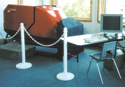
Our bobsled simulator is an electromechanical system that has been designed and constructed to closely mimic the real experience. The driver steers and the simulator calculates how the sled would react. The simulator also provides the driver with sensations similar to those experienced in the actual event. Indeed, it is important to involve as many of the driver’s senses as possible to heighten the feeling of realism. Our bobsled simulator therefore addresses the visual, tactile and auditory senses, as well as the driver’s sense of balance, using both hardware and software.
The heart of the simulator is a high-speed computer that calculates the differential equations that model the dynamics. The driver’s steering is measured with an optical encoder and fed directly to the computer to affect the equations of motion. These equations are solved in real time at 100 Hz. Meanwhile, a continuously changing visual image is generated showing what would be seen by the driver from his or her position on the track.
Although visual feedback accounts for some 70% of the perceived motion, the angular motion of the organs in the inner ear is also important. Sleds experience angular accelerations in all three directions, but the roll component around the forward axis is by far the largest and most violent, with angular accelerations frequently exceeding 60 rad s-2. A DC motor controls the roll of the simulator cockpit to mimic this motion.
Another important factor for drivers is the “feel” of the steering. Our simulator calculates the forces on the runners and those that are transmitted through the steering linkage to the drivers’ hands. We then reproduce these forces using an active DC-motor control system in the steering mechanism to produce realistic tactile sensations. Since the track surfaces are rarely smooth, the interaction between the runners and surface irregularities on the ice produces extremely severe vibrations and auditory noise. A final touch of realism in the simulator is provided by recorded acoustic noise from actual track runs.
Although every effort is made to have accurate and realistic sensory feedback, the simulator does have its limits. For example, bobsledding involves extremely high specific forces, with the team experiencing forces equivalent to five times the acceleration due to gravity for up to 2 seconds at a time. But it is impossible to simulate such accelerations in a cockpit based in the lab, which limits the specific forces to 1g.
Because everything is computed in real time, virtually all the variables of interest can be displayed to the driver after the run to learn what went right and wrong. This is one of the great advantages the simulator has over a real bobsled – it is very expensive and takes immense effort to measure the same variables during real runs. Immediate quantitative feedback to the driver is extremely important to help improve his or her driving technique.
Another great benefit of the simulator is that the driver can practise the runs many times. On a real track, drivers are lucky to make four runs lasting one minute due to competition from other teams wanting to use the same track. Another obvious advantage of the simulator is safety: teams can experiment with driving strategies that would be too risky and dangerous to try in practice.
Improved performance
So has the simulator led to faster times in competitions and more medals? Unfortunately, it is nearly impossible to test the effectiveness of the simulator experimentally. The reason is that the performance of the driver is just one – and perhaps not even the most important – of the three major factors that determine the finish time. The other two – push effectiveness (i.e. the velocity and time at the end of the push) and the aerodynamic and frictional efficiency of the sled – are unrelated to driving skill.
That said, the simulator allows us to completely control factors that are uncontrollable in real races. Differences in the finishing time in the simulator are solely down to driving technique, since all the other conditions are held constant. By measuring these times over long periods, it is clear that the simulator does lead to a gradual improvement in driver performance.
Even though the simulated experience can never completely replace actual sledding, drivers praise its realism, its ability to capture the essential features of driving, and its effectiveness in increasing their familiarity with particular track layouts. So far, our simulator has proved an effective tool in tuning the skills of world-class drivers. And at the other end of the spectrum, the simulator can help to train novice drivers rapidly and safely.
Scully considered a simplified version of the Otto cycle, a sequence of operations similar to that carried out by a standard car engine. In this four-step cycle, a hot gas expands in a cylinder doing useful work before it loses heat to its surroundings; then it is compressed and heated again.
But Scully added two extra steps. After the heat has dissipated the gas is passed through a laser-maser cavity at constant temperature, where it deposits useful energy. This cavity is then reheated once the system as a whole has been reheated, again at a constant temperature.
The crux of Scully’s system is that the heating of the cavity does not raise the kinetic energy of the atoms in the gas, as the normal heating stage does. Instead it increases the internal energy levels of the atoms, making them emit photons. Scully calculated that this liberated quantum energy was greater than the extra work that would have been produced if the additional heat had instead been ploughed into a normal four-stage cycle.
Scully points out that this result does not violate any laws of thermodynamics. He also analysed an equivalent system in a Carnot cycle – which, unlike the Otto cycle, runs at the highest efficiency permitted by thermodynamics – and found that quantum mechanics could not be used to improve the engine’s performance.
He hints that he has already worked out how to test his idea in the lab and that he has conceived several novel laser systems. His idea has been dubbed a ‘quantum afterburner’ because of its parallel with the devices that extract useful energy from the exhaust of a jet engine.
Last year, physicists at the Sudbury Neutrino Observatory in Canada confirmed that neutrinos can ‘oscillate’ from one flavour (electron, muon or tau) to another, and that they therefore have mass. It is not possible to deduce the flavour masses directly from such oscillations, only the difference between them, but the results suggest that the masses lie somewhere between 0.01 and 0.05 eV.
In contrast, Fiorini and co-workers will study a phenomenon known as double-beta decay. This extremely rare form of beta decay, which does not involve the emission of antineutrinos, is only possible if neutrinos have mass and they are their own antiparticles. Although it is extremely unlikely to happen in any one nucleus, such a decay should be seen over the lifetime of the CUORE experiment – which will consist of 1000 cubes of tellurium oxide, each weighing 750 grams. The effective mass of the electron neutrino can then be deduced from the associated decay lifetime.
Current double beta-decay experiments are not large enough to make a direct observation of this rare decay, but they can set a lower limit to the decay half-life and a corresponding upper limit on the neutrino mass. Combining these data with the results from the SuperKamiokande laboratory in Japan, the neutrino mass is tentatively predicted to lie between 0.01 and 1 eV. Results from an experiment involving just 20 tellurium crystals indicate that CUORE should be able to probe down to about 0.02 eV, which would put it in sight of neutrino-less decay.
In the unlikely event that CUORE did not make such an observation, it would still be able to set a much more precise upper limit on the neutrino mass. If this is as low as the results from the oscillation experiments suggest then neutrinos can be ruled out as a significant source of dark matter – to account for all the dark matter in the universe, the neutrino would need to have a mass of between 10 and 50 eV.
CUORE has its rivals, however, including two proposals that would use the material found in the current generation of detectors, germanium-76. But according to the Milan group, these experiments would be more expensive since germanium-76 – unlike tellurium-130 – is a relatively rare isotope that requires enrichment. Fiorini and colleagues point out that in contrast to CUORE these detectors would also need significant R&D. But they add that a sighting of neutrino-less decay made by CUORE would need to be confirmed by a second detector of about the same size built from a different material.
The electrons in a three-dimensional metal can be described as a ‘Fermi liquid’, in which electrostatic – or Coulomb – interactions between the negatively charged particles play only a minor role. But physicists believe that electrons confined to one dimension will behave as a so-called Luttinger liquid, in which Coulomb interactions are much more important. Ophir Auslaender and co-workers studied the quantum mechanical ‘tunnelling’ of electrons between virtually one-dimensional wires to find out if this is true.
‘Understanding how electrons move in a single wire can help us to understand how more complex one-dimensional systems behave’, Auslaender told PhysicsWeb. ‘Recently there have been some attempts to understand high-temperature superconductors based on the physics of these systems.‘
Auslaender’s team made two parallel ‘quantum wires’ from gallium arsenide. The wires were tens of nanometres in diameter, several micrometres long and separated by a six-nanometre insulating barrier of aluminium gallium arsenide. Quantum mechanics allows electrons to ‘tunnel’ from one wire to the other through this barrier.
In order to tunnel between these wires, an electron must have a precise amount of energy and momentum. The energies and momenta of the electrons are controlled by a voltage applied across the wires and a magnetic field applied perpendicular to them.
By measuring how the conductance of the insulating barrier changes as the energy and momentum were adjusted, Auslaender’s team were able to map the excitation spectrum of electrons in one dimension for the first time.
At a certain combination of voltage and momentum, the researchers found that the ‘excitation velocity’ of the electrons was 30% greater than it was for non-interacting electrons. According to Auslaender’s team, this increase is evidence for the significant interactions between electrons moving in one dimension.
‘The one-dimensionality restricts the screening ability of the electrons and renders the mutual interactions very effective’, said Auslaender.
Auslaender and colleagues hope that their technique could lead to the first observation of ‘spin-charge separation’. In this phenomenon – which was predicted in 1968 – electrons confined to one dimension can be excited into states where they have a spin but no charge, or a charge but no spin. The researchers admit that more work is needed, but by mapping the excitation spectrum of a one-dimensional electron system, they could have taken a crucial step towards detection of this exotic effect.