Small companies, especially those built around new technologies, are the flavour of the month in many countries. Small and medium sized enterprises or “SMEs” are said to be quicker than large companies when it comes to bringing new science to market and creating new jobs. The trouble is that SMEs, unlike large companies, rarely have the money to fund their growth.
The venture capital industry is there to provide that cash (see ). Figures from the British Venture Capital Association show that some 295 high-technology companies in the UK received a record £690m of venture capital investment in 1997 – the largest sum for any industry grouping. Despite such large sums being available, physics-based companies can find it difficult to raise capital. It is much easier for investors to back a business built around biotechnology or software, for example. Both sectors have their own specialist funds, not to mention separate categories in stock exchange listings.
It is not so much that investors reject physics. Rather, there is not the track record of success that investors like. There are simply too few examples of ideas that have gone from a university physics department, say, to become major commercial ventures. In comparison, countless academics have biotech and software millionaires.
Someone with fresh wounds from raising funds for physics-based ventures is John Campbell, chief executive of Investech, a small investment company that advises small high-technology firms. Campbell recently played a major part in persuading 3i, Europe’s largest venture capital company, to invest £2m in a small business called Printable Field Emitters. The company hopes to develop field-emission display technology for application in large-area flat TV and information displays (see Physics World June 1997 pp45-48). “It was not easy at all, ” says Campbell of fund raising. “We tried something like 20 or 30 sources of finance and got nowhere. In the end, 3i came up trumps.”
The experience of Printable Field Emitters underlines several important factors. 3i had previously turned down the idea, and only began to think again when experienced directors like Campbell – who recently retired as chief technology officer of Cookson, the high-tech materials company – came on board. Changes in the management of a company may also be necessary. “You need a different type of management to run a company than you do to found it, ” says Campbell.
One problem when it comes to ideas-based companies, says Campbell, is that it can be hard for investors to see where an idea will go, what the market will be, and how to set up production. It is difficult to persuade investors that a handful of patents is valuable and even harder to convince them to put money into completing the science. “It is easier to raise money for businesses that have got a product that the customer is buying, ” he says.
Dave Cheesman agrees with this view. He works for Advent, one of the UK’s leading venture capital funds, and for TriTech Investment Managers, who deal with the smaller investor. “We do look at physics-based businesses, ” says Cheesman, but he acknowledges that it is harder to raise money here than in biotech and software. For a start, he points out, “the gestation time is often very very long” for start-ups in areas such as physics and materials. And some ideas from physicists simply need more money than even the most adventurous investors will cough up. Cheesman talks of one “big ticket” idea that would have needed £50m just to try it out. Only governments can afford this sort of money and it is a waste of time approaching the City for such ventures, he warns.
It can also be difficult to chart the manufacturing steps and processes that a company will need before an idea becomes a product. In areas such as biotechnology, however, the route to market is well-defined. Moreover, the financial returns can be much larger. Physicists and biologists also differ in their attitudes to business, Cheesman believes. “Physicists are less commercial, ” he says. “There are role models in the biotechnology industry who have gone forward and made a lot of money.”
It is not that venture capitalists want to invest only small amounts in an idea, rather that anything less than about £250, 000 is too small to justify the effort needed to assess and monitor a company. This leads to the infamous investment gap. Would-be entrepreneurs can usually get the money needed to fund the first step, but it is much more difficult to raise amounts of between about £50,000 and £250,000
One way to plug the gap is to apply for a SMART award from the government to commercialize an idea for a new product. “I know of companies where [an award] has saved the day, ” says Cheesman. The future of such schemes is currently being discussed following the publication of a consultation document, Innovating for the Future: Investing in R&D, earlier this year. Indeed, the fact that the Department of Trade and Industry and the Treasury worked together on the document is seen as nothing short of a miracle in some circles.
Recent months have seen several government initiatives in this area. The University Challenge fund was announced in March. And in June, the chancellor, Gordon Brown, unveiled a trio of new venture capital funds, worth a total of £240 million, to support small and medium sized businesses (Physics World July p11). However, most of the money for these initiatives is coming from the private sector – either charitable foundations or venture capital firms.
Meanwhile, Sir Peter Williams, chairman of Oxford Instruments, one of the UK’s leading physics-based companies, is chairing a working group that is examining the financing of high-technology companies. Sir Peter promises that the group’s report, due for publication later this year, will offer some radical suggestions on the financing of high-tech companies.
If anyone knows the problems of financing a company with physics at its heart it is Williams. After three days solid telling the City about the company’s results, he threatened to change the company’s name to Oxford Bioinstruments. Williams was joking, of course, but his remark underlines the problems that physics can face in the world of finance.
The past two years have witnessed the strongest El Niño this century. Indeed, the event received so much media coverage that the phrase “El Niño” is now part of our everyday vocabulary. The impact of the 1997/8 El Niño was felt in many parts of the world: floods and warm weather led to a failed anchovy season in Peru; torrential downpours and mud slides besieged southern California; droughts caused uncontrollable forest fires in Indonesia; coral in the Pacific Ocean was bleached by hotter than average water; and shipping through the Panama Canal was restricted by below-average rainfall.
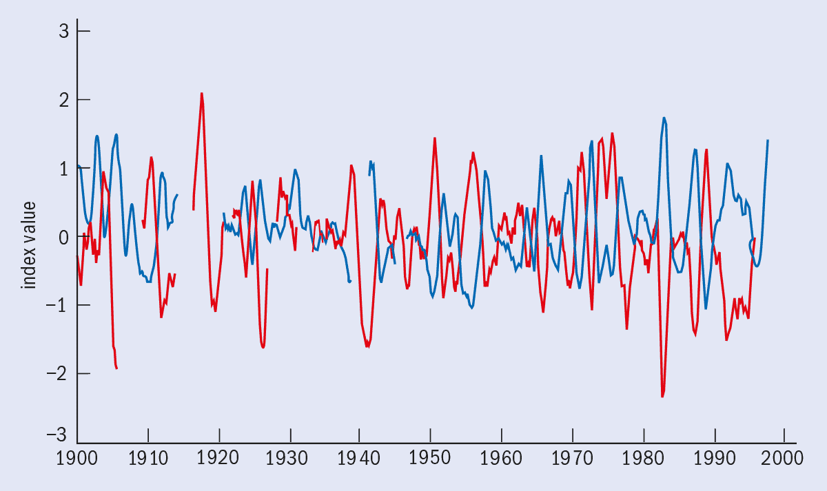
1 A century of El Nino The Southern Oscillation Index (red line) is the sea-level pressure measured at Tahiti minus that measured at Darwin. The CT Index (blue) is the anomaly in the sea-surface temperature averaged over the region between 5° south and 5° north, and between the Date Line and 90° west. The inverse relation between the two indices is clear, as is the variation in the onset, duration and strength of the events. The El Nino events of 1990/4 and 97/8 can be clearly seen.
Long before its global impacts were known, Peruvian fisherman had given the name El Niño to a warm southward current that normally appeared in the first months of each year. Every few years, however, the return of the warm current started earlier, around Christmas, and the fisherman called it El Niño (meaning “the Christ child”).
During the 1960s and 70s, oceanographers used El Niño to refer to an anomalous large-scale warming in the equatorial eastern and central Pacific. At about the same time, scientists began to realize that this warming was intimately linked to an atmospheric phenomenon – the Southern Oscillation – discovered by Sir Gilbert Walker in 1923. The Southern Oscillation is, in simple terms, a “seesaw” of atmospheric pressure between the Pacific and Indian oceans. The clearest sign of the oscillation is the inverse relationship between the air pressure measured at two sites: Darwin, Australia, in the Indian Ocean and the island of Tahiti in the South Pacific. When the air pressure rises in Darwin, it falls in Tahiti, and vice versa.
By the early 1980s it was evident that El Niño and the Southern Oscillation were related, and scientists coined the acronym ENSO to describe this large-scale, interannual climate phenomenon. Various indices have been used to characterize ENSO. The Southern Oscillation Index (SOI) is the difference in sea-level pressure measured at Darwin and Tahiti, while the Cold Tongue (CT) Index measures how much the average sea-surface temperature in the central and eastern equatorial Pacific varies from the annual cycle (figure 1). It is evident that the two indices are anti-correlated, so that a negative SOI is usually accompanied by an anomalously warm ocean – El Niño.
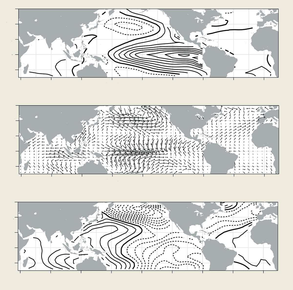
2 Blowing hot and cold The chart shows climate anomalies over the oceans that are associated with a typical warm ENSO event. Sea-surface temperature (top); surface wind stress (middle); and atmospheric sea-level pressure (bottom). The anomalies are measured with respect to the annual climatological cycle. (From Zhang et al.) The solid (dashed) lines are positive (negative) contours at linearly spaced intervals. The warming of the Pacific Ocean in the tropics is particularly obvious.
Although ENSO is inherently caused by interactions between the atmosphere and the ocean in the tropical Pacific, it is responsible for changes in the global climate system that are especially evident throughout the western hemisphere (figure 2). The anomalies that can be seen in the northern Pacific have been shown to be “teleconnected” from the tropics via a large-scale redistribution of vorticity in the atmosphere.
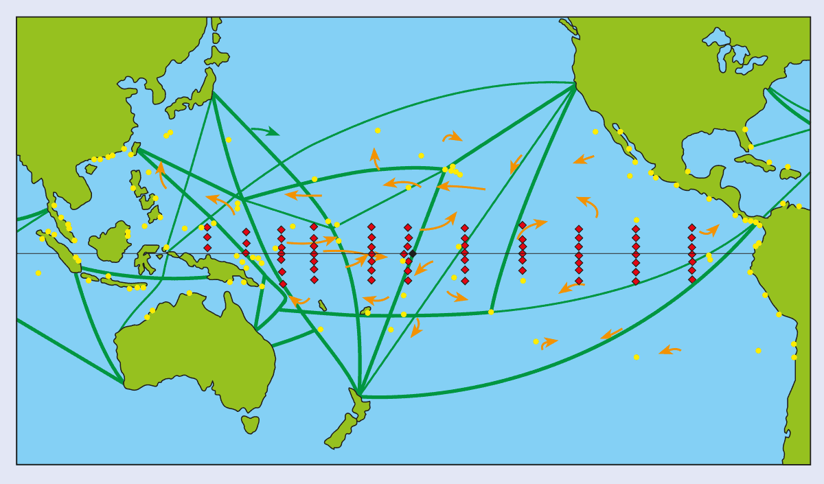
Since recognizing the importance of ocean-atmosphere interactions to ENSO, remarkable progress has been made towards a comprehensive understanding of the phenomenon. An ENSO observing system has been established over the past 10-15 years and we can now observe the state of the upper tropical Pacific Ocean in real time (figure 3). We have also built accurate climatologies of the surface winds and the upper ocean (both its thermal structure and currents), and developed techniques to combine data from sparse observations with simulations, producing historical data sets that are spatially complete and consistent with the laws of physics. Finally, we have constructed coupled ocean-atmosphere models that are capable of simulating many aspects of ENSO.
All this progress means that we are gradually starting to understand the nature of the annual, year-to-year and long-term variability of the Pacific. We have begun to use data from the observing system for operational seasonal-to-interannual climate forecasting, and have demonstrated that the state of the coupled ocean-atmosphere system in the tropics can be predicted several seasons in advance.
Characteristics of ENSO events
Observations show that ENSO is a highly variable phenomenon: events last about 12-18 months and the time between events ranges from two to seven years. The strength also varies greatly from event to event (figure 1). Further analysis indicates that for most warm ENSO events, the maximum warming in the eastern equatorial Pacific occurs in December and January. The following features also seem to be common to most ENSO events.
(a) Quasi-stationary anomalies in the sea-surface temperature (SST) in the eastern and central Pacific.
(b) A relaxation of the trade winds – easterly winds in the tropical Pacific – associated with positive SST anomalies at the onset of the event.
(c) A deepening in the east and a shallowing in the west of the thermocline along the equator. (The thermocline is the zone at the top of the ocean in which the water temperature decreases rapidly with depth.)
(d) Prior to the peak of the ENSO event, the anomalously deep thermocline in the eastern/central Pacific begins to return to normal values.
(e) The trade winds in the far western Pacific increase one or two seasons before the onset of an event.
Despite these common traits, the detailed features of any single ENSO event can vary considerably, including when and where the initial warming starts. For example, sea-surface temperatures near Peru increased by more than 5 ºC during the 1997/8 event. In contrast, in the 1986/7 event the warming extended only as far the mid-Pacific and the maximum temperature was a modest 1 ºC above normal.
Events also vary on longer timescales. During the 1930s and 40s, for example, ENSO events were not as frequent or as severe as those in the past three decades. This irregularity reflects the complexity of the coupled ocean-atmosphere system and hints at the difficulties in predicting ENSO. Therefore, understanding the irregularity of ENSO is a major area of endeavour in climate research.
Understanding ENSO: early ideas
Although it was discovered by Walker in 1920s, the first major breakthrough in understanding the Southern Oscillation and its oceanic counterpart, El Niño, occurred in the 1960s when the Norwegian meteorologist Jacob Bjerknes made two very important discoveries.
First, he noted that the Southern Oscillation is a perturbation to what he called the Walker circulation – a thermally driven east-to-west circulation across the equatorial Pacific. In the Walker circulation, moisture-laden air converges onto the warmest regions of the world’s oceans – the western equatorial Pacific – where it rises and the moisture condenses. This leads to widespread cloudiness and heavy precipitation. In the eastern equatorial Pacific, where the surface water is relatively cold, dry air descends from the upper troposphere and prevents substantial rainfall. In the Walker circulation these motions – rising in the west, sinking in the east – are connected through easterly trade winds near the surface and a westerly wind aloft.
3 Watching the Pacific Ocean The ENSO observing system in the tropical Pacific includes tide gauge stations (yellow circles) that measure sea level, drifting buoys (orange arrows) that measure sea-surface temperature and upper ocean currents, and moored buoys (red diamonds) that measure upper ocean temperature and currents, surface wind and energy flux. Instruments on so-called volunteer ships of opportunity measure the upper ocean temperature and pressure on various sea routes (green lines).
The Southern Oscillation is associated with fluctuations in the intensity and position of the rising moist air, and hence with changes in the prevailing trade winds over the tropical Pacific. Bjerknes was the first to recognize the coupling between changes in the oceanic and atmospheric circulations during ENSO. Based on the observations, he reasoned that the east-to-west increase in the sea-surface temperature in the tropical Pacific and the overlying trade winds were intimately coupled, and that the temperature difference along the equator reinforced the strength of the trade winds.
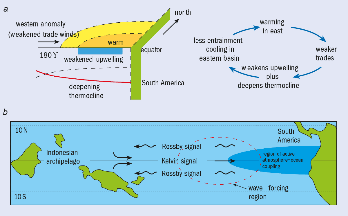
In turn, the easterly wind stress acting on the ocean surface causes the thermocline to rise and the cold subsurface water to upwell in the east. The trade winds and the associated equatorial upwelling maintain the climatological distribution in the sea-surface temperature: a warm pool in the west and a cold “tongue” in the east. However, a modest change in either the equatorial SST or the trade winds can trigger a chain reaction because the ocean and atmosphere are so closely coupled. For instance, if the equatorial trade winds get weaker, the equatorial upwelling will decrease and the thermocline will get deeper, leading to warming in the east and even weaker trade winds (figure 4a). This positive-feedback mechanism, often known as the Bjerknes hypothesis, is believed to be one of the two key ingredients that are responsible for ENSO events.
Bjerknes’ hypothesis laid the foundation for much of the subsequent progress in understanding and modelling ENSO. However, his ideas posed a dilemma: what stops the warming (the positive feedback) in the eastern Pacific? Why do El Niño events typically last only 12-18 months? And why, after about a year, do they usually shut down rapidly and switch to cold conditions?
The middle ages
After Bjerknes’ initial breakthroughs there followed significant theoretical advances in our understanding of how the equatorial ocean responds to wind stress, and of how the atmosphere responds to anomalies in the sea-surface temperature. By the end of the 1960s it was clear that the equatorial region is special: the Coriolis force (which results from the Earth spinning) vanishes at the equator and creates a waveguide in which a variety of waves are trapped to within a few degrees of the equator in the ocean (and a few tens of degrees in the atmosphere). These waves play an important role in determining how the tropical ocean and atmosphere respond to various changes in the surface forcing.
Two types of waves, the equatorial Kelvin and Rossby waves, are of particular importance. Kelvin waves are special gravity waves that propagate eastward with a speed of approximately 2-3 ms-1 in the ocean and have their maximum amplitude at the equator. Rossby waves, which are driven by the variation of the Coriolis force with latitude, propagate westward at about 0.6-0.8 ms-1 near the equator. The oceanic Kelvin and Rossby waves carry energy and momentum received from the wind stress at the ocean surface. They also provide the oceanic “memory” that is so important to year-to-year variability and ENSO.
Rossby and Kelvin waves also exist in the atmosphere, but these move much faster than their oceanic counterparts. This difference in speed means that the tropical atmosphere adjusts to changes in the SST much quicker (10 days or less) than the equatorial ocean responds to changes in wind stress (about six months). The short adjustment time of the atmosphere allows the assumption that the atmosphere is in statistical equilibrium with the SST on timescales longer than a few months. Thus, the long-term memory of the climate system primarily resides in the ocean.
Modelling El Nino and the Southern Oscillation
Advances in modelling the ocean and atmosphere circulations have contributed significantly to our understanding of ENSO. The truly crucial advance was the advent of coupled atmosphere-ocean models. Broadly speaking, the models that have been used to study ENSO can be divided into two types: statistical models and dynamical models based on the laws of physics. Our understanding of ENSO has undoubtedly benefited from both modelling approaches.
Dynamical models can be further divided into three groups. Intermediate coupled models (ICMs) consist of a simple atmosphere model coupled to a simple ocean model. The atmosphere is usually constructed so that winds in the atmospheric boundary layer adjust instantaneously to changes in the SST. The ocean is approximated as immiscible layers of hot and cold water, with changes in the depth of the thermocline between the layers being determined by the conservation laws for mass and momentum. Hybrid coupled models (HCMs) consist of a similar atmosphere coupled to a general circulation model that solves the three-dimensional ocean circulation along with temperature, salinity and other chemical tracers according to the conservation laws for mass and momentum.
Coupled general circulation models (CGCMs) combine general circulation models for both the ocean and the atmosphere. The most complex of the models, CGCMs require extensive computational resources.
In all coupled models, the ocean component must vary with time to allow for the Rossby and Kelvin waves that provide the memory for ENSO. The major difference between simple and general circulation models is in the ability to simulate vertical structure and nonlinear processes in the oceans.
The atmospheric components of the models, on the other hand, differ fundamentally. The simple models capture only a portion of the atmospheric variability that is driven by the SST (sometimes called the “signal”) and ignore completely the portion that is determined by internal atmospheric dynamics, such as hydrodynamic instability and turbulence (the “noise”). In contrast, general circulation models simulate a full spectrum of atmospheric variability, including both the signal and the noise.
Many of the coupled models produce ENSO-like interannual variability through ocean-atmosphere interactions, providing further support to the notion that ENSO is of the coupled atmosphere-ocean system phenomena. However, the simulated interannual variability exhibits a rich variety of behaviour in, for example, the distribution and evolution of temperature anomalies, or the strength and the dominant oscillation period of ENSO cycles. Nevertheless, coupled ocean-atmosphere models have been used extensively to explore the physics of ENSO and to simulate events that evolve via the delayed-oscillator physics.
Meanwhile, simple models (ICMs and HCMs) have been used to explore the importance of nonlinear dynamics in ENSO and identify different dynamical regimes of the coupled system. On the one hand, extensive numerical experiments have shown that the irregularity of ENSO can be generated by a low-order chaotic process due to nonlinear interactions between the annual cycle and interannual oscillation of the coupled system. On the other hand, these same models, when first stabilized by tuning various parameters and then forced by stochastic noise, support ENSO-like variability where self-sustaining oscillations are not possible. Although the character of any natural stochastic noise is unknown at the moment, it is likely that stochastic atmospheric processes provide a major source of ENSO irregularity in nature.
The renaissance
The free, oceanic Kelvin and Rossby waves can be strongly modified by the air-sea coupling. Indeed, the coupling between the ocean and atmosphere generates new wave “modes” with characteristics that depend on the physical processes that control the dynamical and thermodynamical adjustment of the ocean. There are two key timescales for ENSO: one associated with the dynamical adjustment of the equatorial ocean, and the other associated with the changes in the SST due to air-sea coupling.
Two extreme limits are interesting: when the dynamical adjustment of the ocean is either fast or slow compared with the changes in sea-surface temperature. In the fast dynamical limit, the behaviour of the coupled ocean-atmosphere system depends critically on the time evolution of the SST, but is less influenced by the ocean-wave dynamics. In the limit of slow dynamics, the modes that are supported in the coupled ocean-atmosphere system are very similar to free, equatorial ocean waves. These waves provide the memory that allows for an oscillation.
In nature, however, the timescale of the ocean adjustment is comparable with that associated with SST changes due to the air-sea coupling, and the response of the coupled system has a decidedly mixed flavour that is described by a “delayed-oscillator mode”. The behaviour of the ENSO mode can be described by a differential-delay equation for the sea-surface temperature anomaly, T, in the eastern equatorial Pacific (the boxed region in figure 4a) dT /dt = cT – bT (t – t) where t is time and t is the timescale associated with the dynamical adjustment of the ocean basin. The right-hand side of the equation consists of two parts: cT represents the positive feedback proposed by Bjerknes, while bT (t – t) is a delayed negative feedback representing adjustment processes in the ocean (figure 4b).
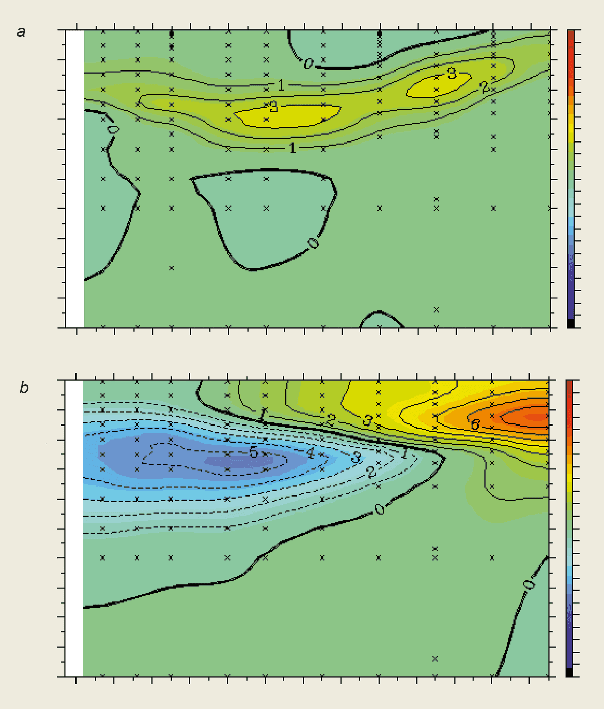
4 Shutting down El Nino Looking down on the ocean from somewhere over the Chilean Andes, (a) In the Bjerknes hypothesis, positive feedback in the interaction between the ocean and atmosphere in the eastern equatorial Pacific leads to a warm ENSO event. The prevailing trade winds are from east to west (right to left). Warming in the central/eastern Pacific region (shown in orange in top panel) is associated with reduced trade winds (westerly anomalies), which deepen the thermocline (red line) in the east and reduce the entrainment of cold subsurface water. This leads to further warming in the east, so the trade winds become weaker and the positive feedback continues (bottom panel). (b) The warm ENSO event shuts down when Rossby waves generated by the relaxation of the trade winds in the central Pacific (red oval) travel west to the Indonesian archipelago and are reflected back as Kelvin waves. The Kelvin waves bring cold water back towards the surface (in the blue region), initiating the cooling that shuts down the warm ENSO event and restrengthens trade winds.
The delayed negative feedback proceeds as follows: although the westerly wind anomaly (in response to warming in the east) deepens the thermocline along the equator, it also causes the thermocline to rise in regions away from the equator (between about 3º and 8º north and south). These off-equator thermocline anomalies propagate stealthily (with respect to the sea-surface temperature) to the west as Rossby wave packets, but otherwise have little effect on the SST.
When the Rossby signals reach the Indonesian archipelago, they are reflected back as Kelvin waves along the equator and cause the thermocline to rise back towards the surface. In the western Pacific, the thermocline is already so deep that the local SST is not affected. In the east, however, the mean upwelling is strong and the thermocline is, on average, much closer to the surface (even during a warm ENSO event). Hence, as the Kelvin signal moves into the eastern Pacific, the thermocline moves even closer to the surface. It is the resultant surface cooling that is responsible for the shutdown of the local Bjerknes positive feedback, and hence the termination of the warm ENSO event.
There is a gap of about six months between the creation of the Rossby waves in the central Pacific and the return of the Kelvin wave to the region. This timescale, t, is comparable with that associated with the local Bjerknes mechanism. It also provides the “memory” of the coupled system that is essential for the shutdown of warm and cold ENSO events, and for the typical transition from warm into cold events – often called La Niña. The delayed-oscillator theory advances our understanding of ENSO because it offers an explanation for the evolution and duration of ENSO events (about one year) and for the tendency (at times) for the system to have perpetual turnarounds from warm to cold states and back again, which the Bjerknes hypothesis cannot explain.
The future
5 In-depth changes Temperature anomalies along the equator from the surface to a depth of 500 m. (a) In February 1997 the deepening thermocline in the eastern and central Pacific is evident from the region of anomalously warm water (yellow) at 100–150 m. This thermocline deepening presages El Nino warming in the summer, (b) At the peak of the event in January 1998 the tongue of anomalously cold water (blue) in the western/central Pacific is about to shut down the event. The 1997/8 ENSO is well described by the delayed-oscillator model.
Is the delayed oscillator the real mechanism for ENSO? Observations are remarkably consistent with the positive-feedback mechanism during the development of an ENSO event. There is also evidence to suggest that the delayed-adjustment processes due to Rossby and Kelvin waves contribute to the termination of a warm event. This year’s ENSO event evolved in a way that was entirely consistent with the delayed-oscillator hypothesis (figure 5).
However, there are inconsistencies between observations and theory during the onset of events. For example, the strengthening of the trade winds that sometimes precedes the event is not a feature of the delayed-oscillator theory. (Since the delayed-oscillator theory views ENSO as a self-sustained regular cycle it is meaningless to discuss whether the cause of ENSO resides in the atmosphere or in the oceans – any small perturbation to either can trigger oscillations in the combined system.)
Some scientists have also questioned the idea that the coupled atmosphere-ocean system is unstable: they argue that the tropical Pacific is a stable system and that the ENSO variability can be viewed as a response of such a system to stochastic processes in the atmosphere. Simulations have suggested that ENSO-like variability can be generated by external random forcing in a globally stable dynamical regime (in which a self-sustained ENSO-like oscillation is not possible). In these models the development of a warm event is interpreted as a constructive interference of stable non-normal modes in the system. An attractive feature of the stochastic theory is that it offers a natural explanation in terms of noise to the irregular behaviour of ENSO variability.
The other competing hypotheses for the ENSO irregularity include nonlinear interactions between ENSO and the seasonal cycle, and the inherent nonlinearity of the coupled system.
Predicting ENSO
Among the greatest achievements in our understanding of ENSO is the establishment of a theoretical foundation for the prediction of short-term climate variability. The quasi-periodic nature of ENSO implies a good deal of predictability. Unlike the weather, which is known to be unpredictable beyond approximately two weeks due to the chaotic nature of the atmosphere, the interannual variability of sea-surface temperatures associated with ENSO can be predicted several seasons – perhaps more than a year – in advance. And because tropical sea-surface temperatures serve as an important boundary condition on the global atmosphere, the ability to predict these offers the possibility of making forecasts of ENSO-related atmospheric anomalies.
The first successful forecast of ENSO was made using an intermediate coupled model developed by Mark Cane and Steve Zebiak at the Lamont-Doherty Geological Observatory of Columbia University in the US. The model successfully predicted the onset of the 1986/7 El Niño one year in advance. Since then, the field of ENSO prediction has grown and there is now a variety of models that have demonstrated skill in forecasting the SST in the central and eastern equatorial Pacific up to a year in advance (see on models). ENSO forecasts are now available in the monthly Climate Diagnostics Bulletin and the quarterly Experimental Long-Lead Forecast Bulletin.
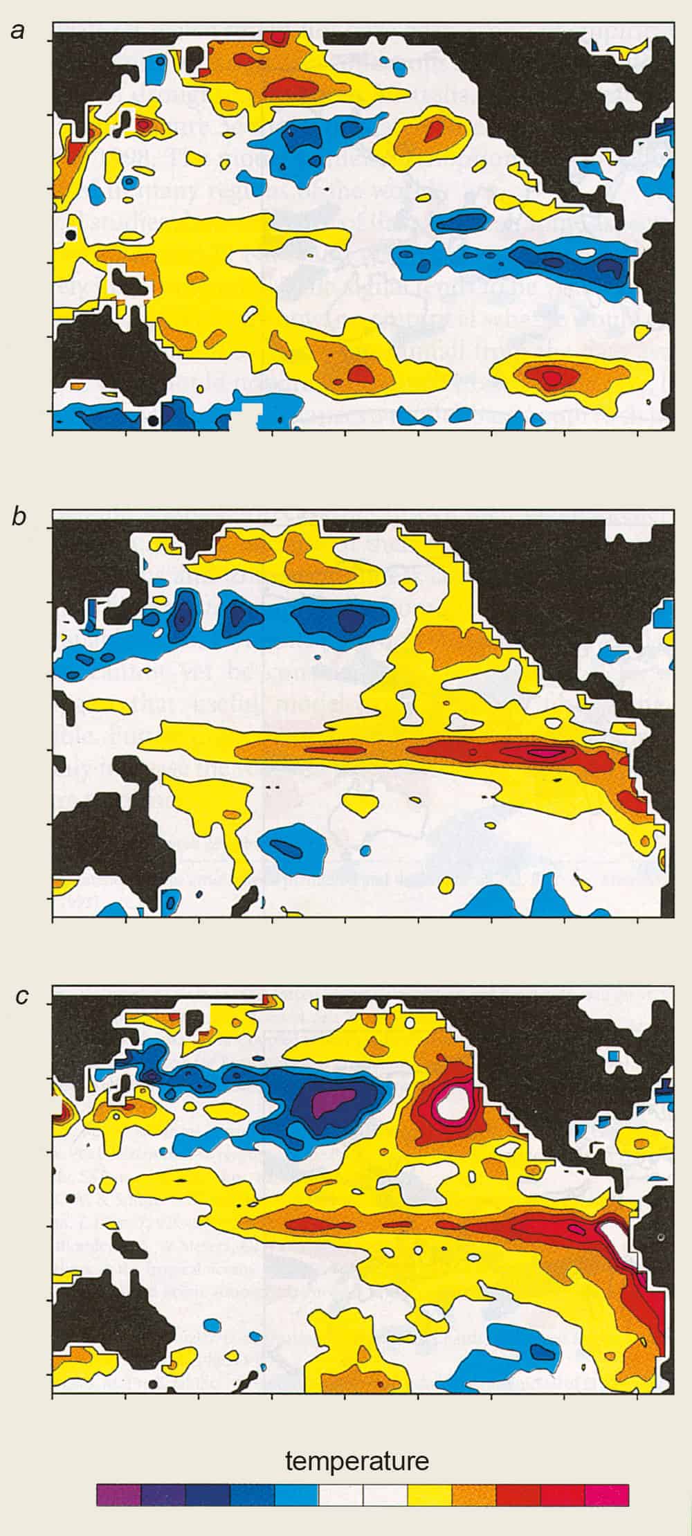
6 El Nino: theory and experiment (a) The sea-surface temperature anomalies in the Pacific in December 1996 that were used to initiate a coupled atmosphere-ocean general circulation model at the ECMWF. (b) The predicted SST distribution for May 1997 is based on an ensemble average of six-month forecasts starting at different days in December 1996 and is in good agreement with what was observed (c). (From Stockdale et al.)
Generally speaking, the statistical models are better than dynamical models for short prediction times (less than six months), but less accurate for longer lead times. This may be partly due to the different initialization procedures used by the models. In an effort to improve the procedures used by dynamical forecast models, various schemes have been developed to use more real data in the simulations. This combination of “data assimilation” and global coupled general circulation models for short-term climate prediction has been implemented in several meteorological centres around the world, including the US National Center for Environment Prediction (NCEP) in Camp Spring, Maryland, and the European Centre for Medium-Range Weather Forecasts (ECMWF) in Reading in the UK. Both the NCEP and the ECMWF systems successfully predicted the onset of 1997/8 El Niño six months in advance (figure 6).
In addition to predicting various winter rainfall patterns commonly associated with ENSO (wet conditions in California, Florida, Uruguay and East Africa, and dry conditions in the Amazon region and southern Africa), the ECMWF model also predicted unexpected weather patterns such as wet conditions in India and southeast China, the absence of drought in northern Australia and the unusually wet climate in western Europe this past winter.
But despite the recent success in predicting the 1997/8 ENSO event, many fundamental questions concerning ENSO predictability remain. What are the dominant physical processes that limit the predictability of ENSO? Are the stochastic processes that are important for the irregularity of ENSO internal to the atmosphere or the ocean? Or are they due to the inherent nonlinearity of the coupled system? Are external forcing and tropical-extratropical interactions responsible for the decadal-to-century modulation of ENSO?
Studies have shown that the skill of many ENSO forecast models drop off considerably when they try to make predictions beyond spring in the northern hemisphere, regardless of when the predictions are made. The dynamical processes that contribute to this “spring predictability barrier” are not clear and we do not know if this is an intrinsic barrier to climate predictions in the tropics. Furthermore, the severity of the barrier appears to undergo a decadal modulation: for instance, the barrier appeared to be stronger in the 1960s and 70s than in the 80s. This decadal modulation may have an effect on the accuracy of model. Finally, most models failed to predict the event that occurred during 1990 to 1994.
Currently, we do not understand why some ENSO events appear to be more predictable than others. Some investigators have speculated that certain events, such as the 1990/4 warming, may be manifestations of a decadal mode in the coupled system with physics that is considerably different to ENSO dynamics. Others believe that stochastic processes play the most important role in determining the predictability of ENSO.
Looking ahead
Much has been accomplished in the past decade in observing, understanding and predicting ENSO. A comprehensive ENSO observing system is in place; models have been developed that simulate ENSO and predict tropical Pacific sea-surface temperature anomalies at lead times of up to a year; and the prospects for seasonal forecasts of short-term climate variability are improving rapidly. Currently, one of the major research activities is to assess how much of this tropical Pacific predictability can be translated into useful climate predictions for the entire globe on seasonal-to-interannual timescales.
Although the impact of ENSO is global, not all anomalous weather patterns are linked to it. In the mid-latitudes, in particular, its effect is small compared with internally generated atmospheric variability. It has also become clear that there are other modes of climate variability – such as monsoons – that have a profound influence on regional climate. Many of these patterns interact with each other (and with ENSO). For example, observational evidence suggests that ENSO is responsible for a portion of the variability of the Asian-Australian Monsoon, and that the temperature variability in the Pacific and Atlantic oceans influences the American Monsoon. Studies also suggest that the variability of the tropical Atlantic basin might have a large impact on the climate over the Americas and Africa. Understanding the multi-basin interactions among the tropical oceans and neighbouring land processes will be a major challenge for future research.
Variability in extratropical climates has also recently received considerable attention. For example, the North Pacific Decadal Oscillation – a strong SST signal that varies on 20-30 year timescale – has a footprint in the north Pacific that is very similar to that due to ENSO (see figure 2). The variability of the North Atlantic Oscillation (NAO) also has a strong influence on the European climate. These mid-latitude climate anomalies are not well understood, although it is generally believed that internal atmospheric variability is important on decadal and longer timescales. Exploration of the basic mechanisms and predictability of decadal climate variability will be an exciting area of future research.
Last, but not least, the effect of global warming due to increases in greenhouse gases and other anthropogenic changes on ENSO is largely unknown. Although coupled general circulation models (GCMs) have been used to study the global-warming scenario, all but one of these models have coarse resolution in the tropics and do not give a realistic representation of ENSO variability. To truly understand the relationship between anthropogenic climate change and natural climate variability, coupled GCMs must achieve accurate simulations of both the natural variability and the response of the climate system to the anthropogenic forcing. Given the complexity of coupled processes in the climate system, this task will be a true challenge to climate researchers for many years to come.
The government plans to invest an extra £400m in new projects through the research councils, £300m in universities through a new Infrastructure Fund and another £300m for research in universities through the regional funding councils. The Wellcome Trust, a medical research charity, is contributing £300m to the Infrastructure Fund and a further £100m towards the construction costs of a new synchrotron X-ray source. Priority will be given to the life sciences and biomedical research, although additional funding is promised for “other priority areas, including the underpinning disciplines of chemistry, engineering, mathematics and physics”. The detailed allocation of the money will be announced later this year.
Physics in the UK will do well to maintain its share of the science budget – currently about 18% – and Ian Halliday, chief executive of the Particle Physics and Astronomy Research Council (PPARC), admits that he feels “slightly nervous about what will happen”. However, there are some grounds for optimism. The government has confirmed that PPARC can spend £104m on building detectors for the Large Hadron Collider at CERN, and a further £13m per year on running costs after 2005. Although not new money, these sums were large enough to require treasury approval. The UK’s world-class astronomy community should now start lobbying to secure funding for its programme.
So how will mainstream physics fare in the scramble for the new money? Physics has been squeezed at the Engineering and Physical Sciences Research Council (EPSRC) since its formation in 1994. When allocating its budget, the council already takes into account how each of the research areas it funds would benefit from additional support, so large increases for physics are unlikely. However, the pressure on physics and related work in materials and other areas at EPSRC should at least be eased.
The money from the Wellcome Trust will also ensure that a third-generation synchrotron radiation source will be built in the UK, probably at the Daresbury Laboratory. Plans for such a facility, DIAMOND, have remained on the drawing board since 1994 because the UK has lacked a system for building large new facilities that will be used by more than one council. With DIAMOND now likely to cost the government less than half the original price, there could be opportunities for other large facilities – such as neutron sources and radioactive beam facilities – to make their cases. And physicists need not lament the fact that they will no longer be the major users of synchrotron radiation. Like X-rays, lasers and magnetic resonance before it, synchrotron radiation should be seen as another spin-off from basic physics into other areas of science.
Overall the increase will be more modest than those mooted for Japan and the US: the “science budget” – essentially the money spent by the UK’s seven research councils – will rise by 24% over three years. But it is still much larger than expected and, more importantly, real rather than hoped-for money. The challenge for physicists and their representatives is to ensure that physics receives as fair a deal as possible when the money is distributed.
The Department of Energy (DOE), which oversees fusion research in the US, wanted to sign the extension. However, the Republican-controlled Congress insisted that the US should not sign it without “Congressional concurrence”. Key members of Congress had such strong doubts about ITER that they withheld their concurrence up to and beyond the deadline.
That struggle now threatens to scupper the whole project. The original ITER agreement said that the collaboration would end if all four parties failed to sign an extension. The lack of an American signature could now terminate the entire ITER project – with potentially serious consequences for the domestic fusion programmes of all four participants.
Last week, ITER’s council met in Vienna, Austria, and cobbled together an agreement that will keep the ITER collaboration going until their next meeting in October. “The US has completed all the formal preparations to sign the extension agreement except for consultations with Congress, ” the DOE said in a statement. The council also agreed on plans suggested by the US that the ITER directorate should set up more formal efforts to work on “lower-cost, reduced-scope options”. And rather than excluding the US from further activity, the four delegations agreed to continue to work together and to maintain the staff at the three ITER sites.
Fred Hoyle was the first to suggest that organic molecules developed in outer space and then fell to the earth, but it was not until the discovery of large quantities of left-handed amino acids in a meteorite last year that biologists seriously started to think about an extraterrestrial origin for the left-handedness of amino acids. If an equal amount of left- and right-handed molecules are bombarded by circularly polarized ultraviolet light, the molecules would take on the same orientation of the light. Although circularly polarized light comes in left- and right-handed version, it is rarely encountered in nature. The Sun, for example, emits unpolarized light.
Bailey et al. observed part of the Orion nebula called OMC-1, a region containing many organic molecules in conditions similar to when the solar system formed. They found that infrared light in this region had been circularly polarised by dust grains. According to their calculations, a similar polarization effect could occur at ultraviolet wavelengths. The observations suggest that the suitability of the Earth for life may be as much a consequence of the environment in which the solar system was formed as of the local conditions on the early Earth.
PEP-II consists of two independent storage rings in the tunnel that housed the original PEP collider. The high-energy ring, which stores a 9 GeV electron beam, is an upgrade of the existing PEP collider, while the low-energy ring, in which the 3.1 GeV positrons are stored, is completely new.
Matter and anti-matter are thought to have been created in equal amounts in the Big Bang, and should have completely annihilated each other. However, we clearly live in a matter-dominated universe, which indicates that a small imbalance must have existed between matter and anti-matter at a very early stage in the universe. PEP-II will make measurements which, physicists hope, will clarify some of the competing theoretical models for this mechanism.
Attempts to locate the satellite with NASA’s Deep Space Network had been unsuccessful. However, by bouncing radio waves from the Arecibo observatory in Puerto Rico off the satellite, and detecting the reflections on a 70 meter radio telescope in Goldstone, California, astronomers have been able to establish SOHO’s position. The signals indicate that the craft is still travelling in its original orbit but rotating at roughly one revolution per minute. However its solar panels are not pointing towards the Sun, which has left SOHO without power.
Engineers expect the solar panels to rotate slowly towards the Sun and hope that by September they will be generating enough power to make communication with the satellite possible. Some of the omens are good. In 1991 ESA recovered a satellite called Olympus under similar circumstances.
Russia and the US each have 50 tons of weapons-grade plutonium to dispose of by either converting it into fuel, or mixing it in with radioactive waste. At the same time, France and the UK separate 20 tons of plutonium a year from spent civilian nuclear fuel but burn only 9 tons a year as reactor fuel. Originally these plants were constructed to provide fuel for nuclear fast-breeder reactors. However, replenished uranium stocks and the expensive construction costs of these fast-breeder reactors has led to a civilian plutonium stockpile. This stockpile – now at 170 tons – is comparable to the amount of military plutonium available. Experts are worried that material from both stockpiles may be stolen by terrorists, or that storing and handling the plutonium will result in an radioactive accident.
However, there may be a solution. Under present commercial arrangements at British Nuclear Fuels Limited (BNFL), the company takes 4, 500 tons of spent light water reactor fuel from its customers and returns 40 tons of reprocessed plutonium, and the equivalent radioactive waste in stored glass containers. Von Hippel suggests that the UK could trade plutonium from its civilian stockpile for this light water reactor waste instead of continuing to reprocess new material. The remnants of the stockpile could then be mixed with liquid high-level waste and glassified, or traded under a similar scheme with Russia. Such a scheme may be attractive to Russia as it recently announced a new $18 billion building programme for several new nuclear reactors, all suitable for burning plutonium. If the UK does not take steps to reduce its stockpile “it will have to resort to much more costly disposal options, ” says von Hippel.
Their technique works by growing single crystal films of the superconducting compound lanthanum-strontium-copper-oxide (La1.9Sr0.1CuO4) on top of a crystal with a smaller lattice spacing. Because the layers are very thin, the layer of superconductor is placed under ‘epitaxial’ strain. The compression in a single plane produces much greater improvements in Tc than standard ways of applying pressure.
If the same techniques can be applied to the compounds with the highest transition temperatures, the authors believe their method has the potential to raise Tc beyond 200 K, a feat they hope might reignite the race towards room-temperature superconductivity.
The charges are designed to help fund the soaring costs of international Internet access from the UK. Over the past four years access costs have risen from £1 million ($1.7 m) to £7 million ($11.1 m). However, the speed at which UKERNA has introduced charging has caught many departments by surprise. UKERNA calls the new fees “token charges” and hints that, in the future, different levels of bandwidth speed will be charged at different rates. Under the new scheme, for example, there is no access charges between 1am and 6am.
UKERNA hopes to raise between £2.2 and £2.6 million from the charges – about 10 percent of its annual budget. And in the long term the organization hopes to receive over 30 percent of its income from charging.