Quantum physics is being transformed by a radical new conceptual and experimental approach known as weak measurement that can do everything from tackling basic quantum mysteries to mapping the trajectories of photons in a Young’s double-slit experiment. Aephraim Steinberg, Amir Feizpour, Lee Rozema, Dylan Mahler and Alex Hayat unveil the power of this new technique

“There is no quantum world,” claimed Niels Bohr, one of the founders of quantum mechanics. This powerful theory, though it underlies so much of modern science and technology, is an abstract mathematical description that is notoriously difficult to visualize – so much so that Bohr himself felt it a mistake to even try. Of course, there are rules that let us extract from the mathematics some predictions about what will happen when we make observations or measurements. To Bohr, the only real task of physics was to make these predictions, and the hope of actually elucidating what is “really there” when no-one is looking was nonsense. We know how to predict what you will see if you look, but if you do not look, it means nothing to ask “What would have happened if I had?”.
The German theorist Pascual Jordan went further. “Observations,” he once wrote, “not only disturb what is to be measured, they produce it.” What Jordan meant is that the wavefunction does not describe reality, but only makes statistical predictions about potential measurements. As far as the wavefunction is concerned, Schrödinger’s cat is indeed “alive and dead”. Only when we choose what to measure must the wavefunction “collapse” into one state or another, to use the language of the Copenhagen interpretation of quantum theory.
Over the last 20 years, however, a new set of ideas about quantum measurement has little by little been gaining a foothold in the minds of some physicists. Known as weak measurement, this novel paradigm has already been used for investigating a number of basic mysteries of quantum mechanics. At a more practical level, it has also been used to develop new methods for carrying out real-world measurements with remarkable sensitivity. Perhaps most significantly in the long run, some researchers believe that weak measurements may offer a glimmer of hope for a deeper understanding of whatever it is that lies behind the quantum state.
Quantum measurement theory
Before quantum mechanics was established, no-one seemed to feel the need for a distinct theory of measurement. A measuring device was simply a physical system like any other, and was described according to the same physical laws. When, for example, Hans Christian Ørsted discovered that current flowing in a wire caused a compass needle to move, it was natural to use this fact to build galvanometers, in which the deflection of the needle gives us some information about the current. By calibrating the device and using our knowledge of electromagnetism, we can simply deduce the size of the current from the position of the needle. There is no concept of an “ideal” measurement – every measurement has uncertainty, and may be influenced by extraneous factors. But as long as the current has had some effect on the needle then, if we are careful, we can look at the needle and extract some information about the current.
Quantum theory, however, raises some very thorny questions, such as “What exactly is a measurement?” and “When does collapse occur?”. Indeed, quantum mechanics has specific axioms for how to deal with measurement, which have spawned an entire field known as quantum-measurement theory. This has, however, created a rather regrettable situation in which most people trained today in quantum mechanics think of measurement as being defined by certain mathematical rules about “projection operators” and “eigenvalues”, with the things experimentalists call “measurements” being nothing more than poor cousins to this lofty theory. But physics is an experimental science. It is not the role of experiment to try to come as close as possible to some idealized theory; it is the role of theory to try to describe (with idealizations when necessary) what happens in the real world.
Such a theory was in fact worked out in 1932 by the Hungarian theorist John von Neumann, who conceived of a measurement as involving some interaction between two physical objects – “the system” and “the meter”. When they interact, some property of the meter – say, the deflection of a galvanometer needle – will change by an amount proportional to some observable of the system, which would, in this case, be the current flowing through the wire. Von Neumann’s innovation was to treat both the system and the meter fully quantum-mechanically, rather than assuming one is classical and the other quantum. (Strange as it may seem, it is perfectly possible to describe a macroscopic object such as a galvanometer needle in terms of quantum mechanics – you can, for instance, write down a “wavepacket” describing its centre of mass.) Once this step is taken, the same theory that describes the free evolution of the system can also be used to calculate its effect on the meter – and we have no need to worry about where to place some magical “quantum–classical borderline”.
This leads to a wrinkle, however. If the meter itself is quantum-mechanical, then it obeys the uncertainty principle, and it is not possible to talk about exactly where its needle is pointing. And if the needle does not point at one particular mark on the dial – if it is rather spread out in some broad wavepacket – then how can we hope to read off the current? Von Neumann imagined that in a practical setting, any measuring device would be macroscopic enough that this quantum uncertainty could be arranged to be negligible. In other words, he proposed that a well-designed observation would make use of a needle that, although described by a wave packet with quantum uncertainty, had a very small uncertainty in position. Provided that this uncertainty in the pointer position was much smaller than the deflection generated through the measurement interaction, that deflection could be established reasonably accurately – thus providing us with a good idea of the value of the quantity we wished to measure.
But the small uncertainty in the position of the needle automatically means that it must have a very large momentum uncertainty. And working through the equations, one finds that this momentum uncertainty leads to what is often referred to as an “uncontrollable, irreversible disturbance”, which is taken by the Copenhagen interpretation to be an indispens-able by-product of measurement. In other words, we can learn a lot about one observable of a system – but only at the cost of perturbing another. This measurement disturbance is what makes it impossible to reconstruct the full history of a quantum particle – why, for example, we cannot plot the trajectory of a photon in a Young’s double-slit experiment as it passes from the slit to the screen. (Actually, as explained in “Weak insights into interference” below, it turns out that weak measurement provides a way of plotting something much like a trajectory.)
Enter weak measurement
The idea of weak measurement was first proposed by Yakir Aharonov and co-workers in two key papers in 1988 and 1990 (Phys. Rev. Lett. 60 1351 and Phys. Rev. A 41 11). Their idea was to modify Von Neumann’s prescription in one very simple but profound way. If we deliberately allow the uncertainty in the initial pointer position (and hence the uncertainty in the measurement) to be large, then although no individual measurement on a single pointer will yield much information, the disturbance arising from a measurement can be made as small as desired. At first sight, extracting only a tiny bit of information from a measurement might seem to be a strange thing to do. But as is well known to anyone who has spent hours taking data in an undergraduate laboratory – not to mention months or years at a place like CERN – a large uncertainty on an individual measurement is not necessarily a problem. By simply averaging over enough trials, one can establish as precise a measure as one has patience for; at least until systematic errors come to dominate. Aharonov called this a weak measurement because the coupling between the system and the pointer is assumed to be too weak for us to resolve how much the pointer shifts by on just a single trial.
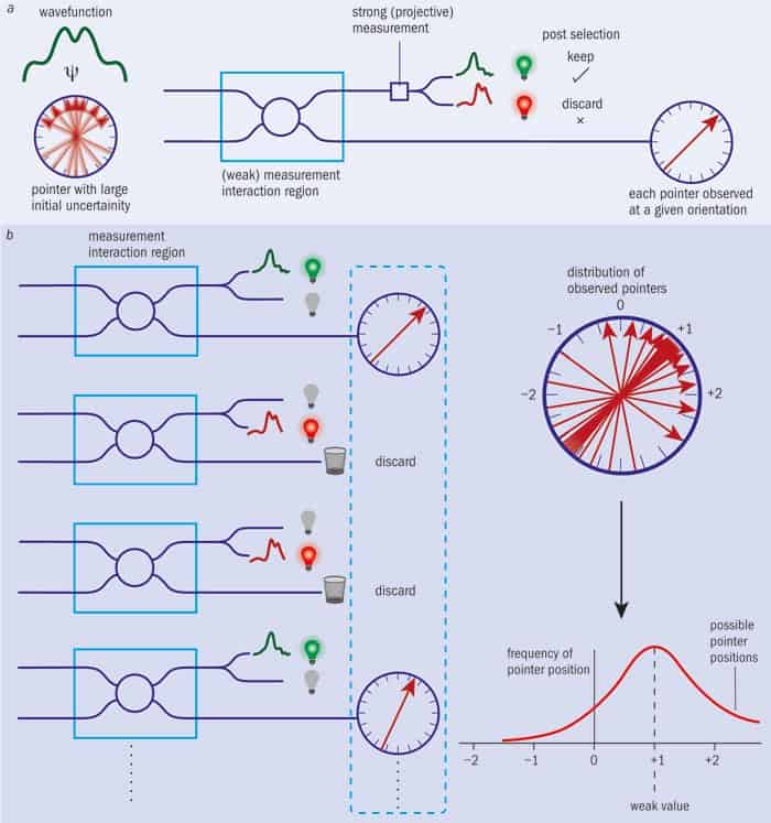
Under normal circumstances, the result of a weak measurement – the average shift of pointers that have interacted with many identically prepared systems – is exactly the same as the result of a traditional or “strong” measurement. It is, in other words, the “expectation value” we are all taught to calculate when we learn quantum theory. However, the low strength of the measurement offers a whole new set of insights into the quantum world by providing us with a clear operational way to talk about what systems are doing between measurements. This can be understood by considering a protocol known as post-selection (see figure 1).
To see what post-selection is all about, let’s consider a simple experiment. Suppose we start at time t = 0 by placing some electrons as precisely as we can at position x = 0. We know from Heisenberg’s uncertainty principle that their velocity will be enormously uncertain, so we will have essentially no idea where an electron will be after, say, 1 second. But if we place a detector 1 metre away at x = 1, any given electron will always have some chance of being spotted there at t = 1 because the wavepacket has spread out over all space. However, when we make a measurement of where the wavepacket is, it may collapse to be at x = 1, or to be elsewhere.
Now suppose we take one of these electrons that appeared at x = 1, which is what we mean by post-selection, and ask ourselves how fast it had been travelling. Anyone with common sense would say that it must have been going at about 1 m/s, since it got from x = 0 to x = 1 in 1 s. Yet anyone well trained in quantum mechanics knows the rules: we cannot know the position and the velocity simultaneously, and the electron did not follow any specific trajectory from x = 0 to x = 1. And since we never directly measured the velocity, we have no right to ask what that value was.
To see why Bohr’s followers would not accept the seemingly logical conclusion that the electron had been travelling at 1 m/s, imagine what would happen if you decided to measure the velocity after releasing the electron at x = 0 but before looking for it at x = 1. At the moment of this velocity measurement, you would find some random result (remember that the preparation ensured a huge velocity uncertainty). But the velocity measurement would also disturb the position – whatever velocity you find, the electron would “forget” that it had started at x = 0, and end up with the same small chance of appearing at x = 1 no matter what velocity your measurement revealed. Nothing about your measurement would suggest that the electrons that made it to x = 1 were any more or less likely to have been going at 1 m/s than the electrons that did not.
But if you do a weak enough measurement of the velocity – by using some appropriate device – you reduce the disturbance that the measurement makes on the position of the electron to nearly zero. So if you repeat such a measurement on many particles, some fraction of them (or “subensemble”, to use the jargon) will be found at the x = 1 detector a second later. To ask about the velocity of the electrons in this subensemble, we can do what would be natural for any classical physicist: instead of averaging the positions of all the pointers, average only the subset that interacted with electrons successfully detected at x = 1.
The formalism of weak values provides a very simple formula for such “conditional measurements”. If the system is prepared in an initial state |i〉 and later found in final state |f〉, then the average shift of pointers designed to measure some observable A will correspond to a value of 〈f|A|i〉/〈f|i〉, where 〈f|i〉 is the overlap of initial and final states. If no post-selection is performed at all (i.e. if you average the shifts of all the pointers, regardless of which final state they reach), this reduces to the usual quantum-mechanical expectation value 〈i|A|i〉. Without the post-selection process, weak measurement just agrees with the standard quantum formalism; but if you do post-select, weak measurement provides something new.
If you work this formula out for the case we have been discussing, you find that the electrons that reached x = 1 were indeed going at 1 m/s on average. This in no way contradicts the uncertainty principle – you cannot say precisely how fast any individual particle was travelling at any particular time. But it is striking that we now know that the average result of such a measurement will yield exactly what common sense would have suggested. What we are arguing – and this admittedly is a controversial point – is that weak measurements provide the clearest operational definition for quantities such as “the average velocity of the electrons that are going to arrive at x = 1″. And since it does not matter how exactly you do the measurement, or what other measurements you choose to do in parallel, or even just how weak the measurement is, it is very tempting to say that this value, this hypothetical measurement result, is describing something that’s “really out there”, whether or not a measurement is performed. We should stress: this is for now only a temptation, albeit a tantalizing one. The question of what the “reality” behind a quantum state is – if such a question is even fair game for physics – remains a huge open problem.
Two-slit interferometers
The possibility of studying such subensembles has made weak measurements very powerful for investigating long-standing puzzles in quantum mechanics. For instance, in the famous Young’s double-slit experiment, we cannot ask how any individual particle got to the screen, let alone which slit it traversed, because if we measure which slit each particle traverses, the interference pattern disappears. Richard Feynman famously called this “the only mystery” in quantum mechanics (see “Weak insights into interference” below).
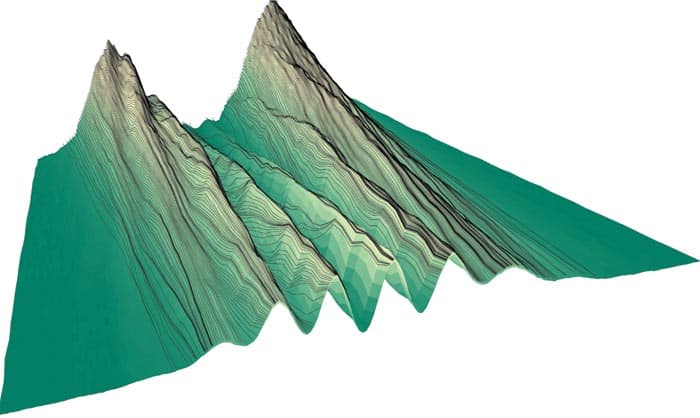
However, in 2007 Howard Wiseman at Griffith University in Brisbane, Australia, realized that because of the ability of weak measurements to describe subensembles we can ask, for instance, what the average velocity of particles reaching each point on the screen is, or what their average position was at some time before they reached that point on the screen. In fact, in this way, we can build up a set of average trajectories for the particles, each leading to one point on the final interference pattern. It is crucial to note that we cannot state that any individual particle follows any one of these trajectories. Each point on a trajectory describes only the average position we expect to find if we carry out thousands or millions of very uncertain measurements of position, and post-select on finding the particle at a later point on the same trajectory.
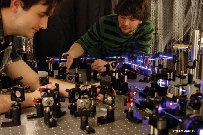
Our group at the University of Toronto has actually carried out this particle-trajectory experiment on single photons sent through an interferometer, which then combine to create an archetypal Young’s double-slit interference pattern. Our photons, which all had the same wavelength, were generated in an optically pumped quantum dot before being sent down two arms of the interferometer and then being made to recombine, with their interference pattern being recorded on a CCD camera. Before the photons reached the screen, however, we sent them through a piece of calcite, which rotates their polarization by a small amount that depends on the direction the photon is travelling in. So by measuring the polarization shift, which was the basis of our weak measurement, we could calculate their direction and thus (knowing they are travelling at the speed of light) determine their velocity. The polarization of the transmitted photon in effect serves as the “pointer”, carrying some information about the “system” (in this case, the photon’s velocity). We in fact measured the polarization rotation at each point on the surface of the CCD, which gave us a “conditional momentum” for the particles that had reached that point. By adjusting the optics, we could repeat this measurement in a number of different planes between the double slit and the final screen. This enabled us to “connect the dots” and reconstruct a full set of trajectories (Science 332 1170) as shown in figure 1.
Back to the uncertainty principle
Throughout this article, we have made use of the idea that any measurement of a particle must disturb it – and the more precise the measurement, the greater the disturbance. Indeed, this is often how Heisenberg’s uncertainty principle is described. However, this description is flawed. The uncertainty principle proved in our textbooks says nothing about measurement disturbance but, rather, places limits on how precisely a quantum state can specify two conjugate properties such as position, x, and momentum, p, according to Heisenberg’s formula ΔxΔp ≥ ħ/2, where ħ is Planck’s constant divided by 2π. But as Masanao Ozawa from Tohoku University in Japan showed in 2003, it is also possible to calculate the minimum disturbance that a measurement must impart (Phys. Rev. A 67 042105). As expected, Ozawa found that the more precise a measurement the more it must disturb the quantum particle. Surprisingly, however, the detailed values predicted by his result said that it should be possible to make a measurement with less disturbance than predicted by (inappropriately) applying Heisenberg’s formula to the problem of measurement disturbance.
At first, it seemed unclear whether one could conceive of an experimental test of Ozawa’s new relationship at all. To establish, for example, the momentum disturbance imparted by measuring position, you would need to ascertain what this momentum was before the position measurement ħ and then again afterwards to see by how much it had changed. And if you did this by performing traditional (strong) measurements of momentum, those measurements themselves would disturb the particle yet again, and Ozawa’s formula would no longer apply. Nevertheless, two teams of researchers have recently been able to illustrate the validity of Ozawa’s new relationship (and the failure of Heisenberg’s formula for describing measurement disturbance). One experiment, carried out in 2012 by a team at the Vienna University of Technology (Nature Phys. 8 185), relied on a tomographic-style technique suggested by Ozawa himself in 2004, while the other by our group at Toronto (Phys. Rev. Lett. 109 100404) used weak measurement, as suggested by Wiseman and his co-worker Austin Lund in 2010, to directly measure the average disturbance experienced by a subensemble.
Uncertainty in the real world
Weak measurements not only provide unique tools for answering fundamental physical questions, but also open new directions in practical real-world applications by improving measurement precision. Remember that the average pointer shifts predicted for weak measurements are inversely proportional to 〈f|i〉, the overlap of the initial and final states. So if the overlap is small, the pointer shift may be extremely large – larger than could ever occur without post-selection. This idea of “weak value amplification” has in fact been used to perform several extremely sensitive measurements, including one by Onur Hosten and Paul Kwiat at the University of Illinois at Urbana-Champaign to measure the “spin Hall” effect of light (Science 319 787) and another by John Howell’s group at the University of Rochester in New York (Phys. Rev. Lett. 102 173601), in which the angle of photons bouncing off a mirror was measured to an accuracy of 200 femtoradians.
Of course, there is a price to pay. By adjusting the overlap between initial and final states to be very small, you make the probability of a successful post-selection tiny. In other words, you throw out most of your photons. But on the rare occasions when the post-selection succeeds, you get a much larger result than you otherwise would have. (Howell’s group typically detected between about 1% and 6% of photons.) Going through the maths, it turns out this is a statistical wash: under ideal conditions, the signal-to-noise ratio would be exactly the same with or without the post-selection. But conditions are not always ideal – certain kinds of “technical noise” do not vary quickly enough to be averaged away by simply accumulating more photons. In these cases, it turns out that post-selection is a good bet: in return for throwing away photons that were not helping anyway, you can amplify your signal (Phys. Rev. Lett. 105 010405 and 107 133603). In fact, measurements enhanced by weak-value amplification are now attracting growing attention in many fields including magnetometry, biosensing and spectroscopy of atomic and solid-state systems.
As often happens in physics, something that began as a quest for new ways to define answers to metaphysical questions about nature has led not only to a deeper understanding of the quantum theory itself, but even to the promise of fantastic new technologies. Future metrology techniques may be much in debt to this abstract theory of weak measurement, but one should remember that the theory itself could never have been devised without asking down-to-earth questions about how measurements are actually done in the laboratory. Weak measurements are yet another example of the continual interplay between theory and experiment that makes physics what it is.
Weak insights into interference
In the famous Bohr-Einstein debates, the fact that an interference pattern in a double-slit experiment disappears if you measure which slit the particle goes through was explained in terms of the uncertainty principle. Measuring the particle disturbs its momentum, the argument went, which washes out the interference. However, from a modern perspective, information is fundamental and what destroys the interference is knowing which slit the photon goes through – in other words, the presence of “which-path” information. In the 1990s there was a rather heated debate over whether or not a which-path measurement could be carried out without disturbing the momentum (see, for instance, Nature 351 111 and 367 626). However, in 2003 Howard Wiseman at Griffith University in Brisbane came up with a proposal to observe what really happens when a measurement is performed to tell which slit the photon traverses (Phys. Lett. A 311 285) – an experiment that our group at the University of Toronto performed for real in 2007 using the principle of weak measurement. We were able to directly measure the momentum disturbance by making a weak measurement of each photon’s momentum at early times, and then measuring strongly what its momentum was at the end of the experiment – the difference between the two values being the average momentum change, roughly speaking (New J. Phys. 9 287).
In the original 1990s debate, the two camps had chosen very different definitions of momentum transfer, leading each to prove seemingly contradictory conclusions about its magnitude. Our experiment, by following Wiseman’s proposal of weak measurement as an operational definition, was thus introducing a third notion of momentum transfer. Remarkably, the result of this experiment agreed with the most important aspects of both original proofs, in some sense resolving the controversy. Even though the different groups chose different definitions, one cannot help but think that all these definitions reveal part of a bigger story about what is really “going on” – otherwise, why should a measurement carried out using one definition satisfy theorems proved for two entirely unrelated definitions? This is just one of the open questions that those who deal with weak measurements find so fascinating.