From sticks in the ground to caesium atomic clocks, humans have been keeping track of time with increasing accuracy for millennia. Helen Margolis looks at how we reached our current definition of the second, and where clock technology is going next
On 1 November 2018, when this article was first published in the print edition of Physics World, I had been working at the UK’s National Physical Laboratory (NPL) in Teddington for exactly 20 years and six days. The reason I know this is easy – I joined on 26 October 1998 and, with the help of clocks and calendars, I can measure the time that’s passed. But what did people do before clocks came about? How did they measure time?
Over the millennia a myriad of devices has been invented for timekeeping, but what they all have in common is that they depend on natural phenomena with regular periods of oscillation. Timekeeping is simply a matter of counting these oscillations to mark the passage of time.
For much of history, the chosen periodic phenomenon was the apparent motion of the Sun and stars across the sky, caused by the Earth spinning about its own axis. One of the earliest known timekeeping methods – dating back thousands of years – involved placing a stick upright in the ground and keeping track of its moving shadow as the day progressed. This method evolved into the sundial, or shadow clock, with markers along the shadow’s path dividing the day into segments.
However, sundials are useless unless the Sun is shining. That’s why mechanical devices – such as water clocks, candle clocks and hourglasses – were developed. Then, in the 17th century, pendulum clocks were developed, which were far more accurate than any preceding timekeeping devices. Their period of oscillation (in the lowest-order approximation) was determined by the acceleration due to gravity and the length of the pendulum. Because this period is far shorter than the daily rotation of the Earth, time could be subdivided into much smaller intervals, making it possible to measure seconds, or even fractions of a second.
Nevertheless, the Earth’s rotation was still the “master clock” against which other clocks were calibrated and adjusted on a regular basis.
From crystal to atomic
As technology progressed, the need for higher-resolution timing increased. Pendulum clocks were gradually overtaken by quartz clocks, the first of which was built in 1927 by Warren Marrison and Joseph Horton at the then Bell Telephone Laboratories in the US. In these devices, an electric current causes a quartz crystal to resonate at a specific frequency that is far higher than a pendulum’s oscillations.
The frequency of such clocks is less sensitive to environmental perturbations than older timekeeping devices, making them more accurate. Even so, quartz clocks rely on a mechanical vibration whose frequency depends on the size, shape and temperature of the crystal. No two crystals are exactly alike, so they have to be calibrated against another reference – this was the Earth’s period of rotation, with the second being defined as a 1/86,400th of the mean solar day (see box, below).
Standardizing time
Solar time is not the same everywhere. In the UK, for example, Birmingham is eight minutes behind London, and Liverpool is 12 minutes behind. While communication and travel times between major centres of population were slow, this mattered little. But the situation changed dramatically with the construction of railways in the 19th century. Having different local times at each station caused confusion and increasingly, as the network expanded, accidents and near misses. A single standardized time was needed.
The Great Western Railway led the way in 1840 and “railway time” was gradually taken up by other railway companies over the subsequent few years. Timetables were standardized to Greenwich Mean Time (GMT), and by 1855 time signals were being transmitted telegraphically from Greenwich across the British railway network. However, it was not until 1880 that the role of GMT as a unified standard time for the whole country was established in legislation. Four years later, at the International Meridian Conference held in Washington DC in the US, GMT was adopted as the reference standard for time zones around the globe and the second was formally defined as a fraction (1/86,400) of the mean solar day.
There are problems with this definition of the second, however. As our ability to measure this unit of time improved, it became clear that the Earth’s period of rotation is not constant. The period is not only gradually slowing down due to tidal friction, but also varies with the season and, even worse, fluctuates in unpredictable ways.
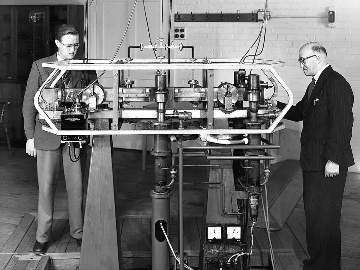
In 1955 NPL set in motion a revolution in timekeeping when Louis Essen and Jack Parry produced the first practical caesium atomic frequency standard (see box, below). Their device was not truly a clock as it did not run continuously, and was simply used to calibrate the frequency of an external quartz clock at intervals of a few days. Nevertheless, by studying how the resonance frequency depended on environmental conditions, Essen and Parry had shown convincingly that transitions between discrete energy levels in well-isolated caesium atoms could provide a much more stable time-interval reference than any standard based on the motion of astronomical bodies. As Essen later wrote: “We invited the director [of NPL] to come and witness the death of the astronomical second and the birth of atomic time.”
How an atomic clock works
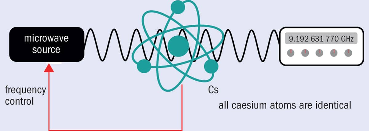 In a caesium atomic clock, the frequency of a microwave source is carefully adjusted until it hits the resonance frequency corresponding to the energy difference between the two ground-state hyperfine levels of the caesium atoms: 9,192,631,770 Hz. The atoms absorb the microwave radiation, and a feedback signal generated from the absorption signal is used to keep the microwave source tuned to this highly specific frequency. The time display is generated by counting electronically the oscillations of the microwave source.
Louis Essen’s original clock at the UK’s National Physical Laboratory used a thermal beam of caesium atoms and was accurate to about one part in 1010. Nowadays, caesium primary standards use an arrangement known as an “atomic fountain”, in which laser-cooled atoms are launched upwards through a microwave cavity before falling back under gravity. Using cold atoms means the interaction time can be far longer than in a thermal beam clock, giving much higher spectral resolution. With careful evaluation of systematic frequency shifts arising from environmental perturbations, today’s best caesium fountains have reached accuracies of one part in 1016, though measurements must be averaged over several days to reach this level. They contribute as primary standards to International Atomic Time (TAI).
But showing that the new standard was stable was insufficient to redefine the second. A new definition had to be consistent with the old one within the technical limit of measurement uncertainty. Essen and Parry therefore proceeded to measure the frequency of their caesium standard relative to the astronomical timescale disseminated by the Royal Greenwich Observatory.
In the meantime, astronomers had switched to using ephemeris time, based on the orbital period of the Earth around the Sun. Their rationale was that it is more stable than the Earth’s rotation, but unfortunately for most practical measurement purposes it is impractically long. Nevertheless, the International Committee for Weights and Measures followed their lead, and in 1956 selected the ephemeris second to be the base unit of time in the International System of Units. As Essen put it: “Even scientific bodies can make ridiculous decisions.”
But ridiculous or not, he needed to relate the caesium frequency to the ephemeris second, a task he accomplished in collaboration with William Markowitz from the United States Naval Observatory. Finally, in 1967 the General Conference on Weights and Measures decided that the time had come to redefine the second as “the duration of 9,192,631,770 periods of the radiation corresponding to the transition between the two hyperfine levels of the ground state of the caesium-133 atom”.
The next generation
More compact and less costly – albeit less accurate – versions of caesium atomic clocks have also been developed, and applications have flourished. We may not always realize it, but precision timing underpins many features of our daily lives. Mobile phones, financial transactions, the Internet, electric power and global navigation satellite systems all rely on time and frequency standards.
But although the caesium transition has proved an enduring basis for the definition of the second, caesium atomic clocks may now be reaching the limit of their accuracy and improvements may open up new applications. In response, a new generation of atomic clocks is emerging based on optical, rather than microwave, transitions. These new clocks get their improved precision from their much higher operating frequencies. All other things being equal, the stability of an atomic clock is proportional to its operating frequency and inversely proportional to the width of the electronic transition. In practice, though, the stability also depends on the signal-to-noise ratio of the atomic absorption feature.
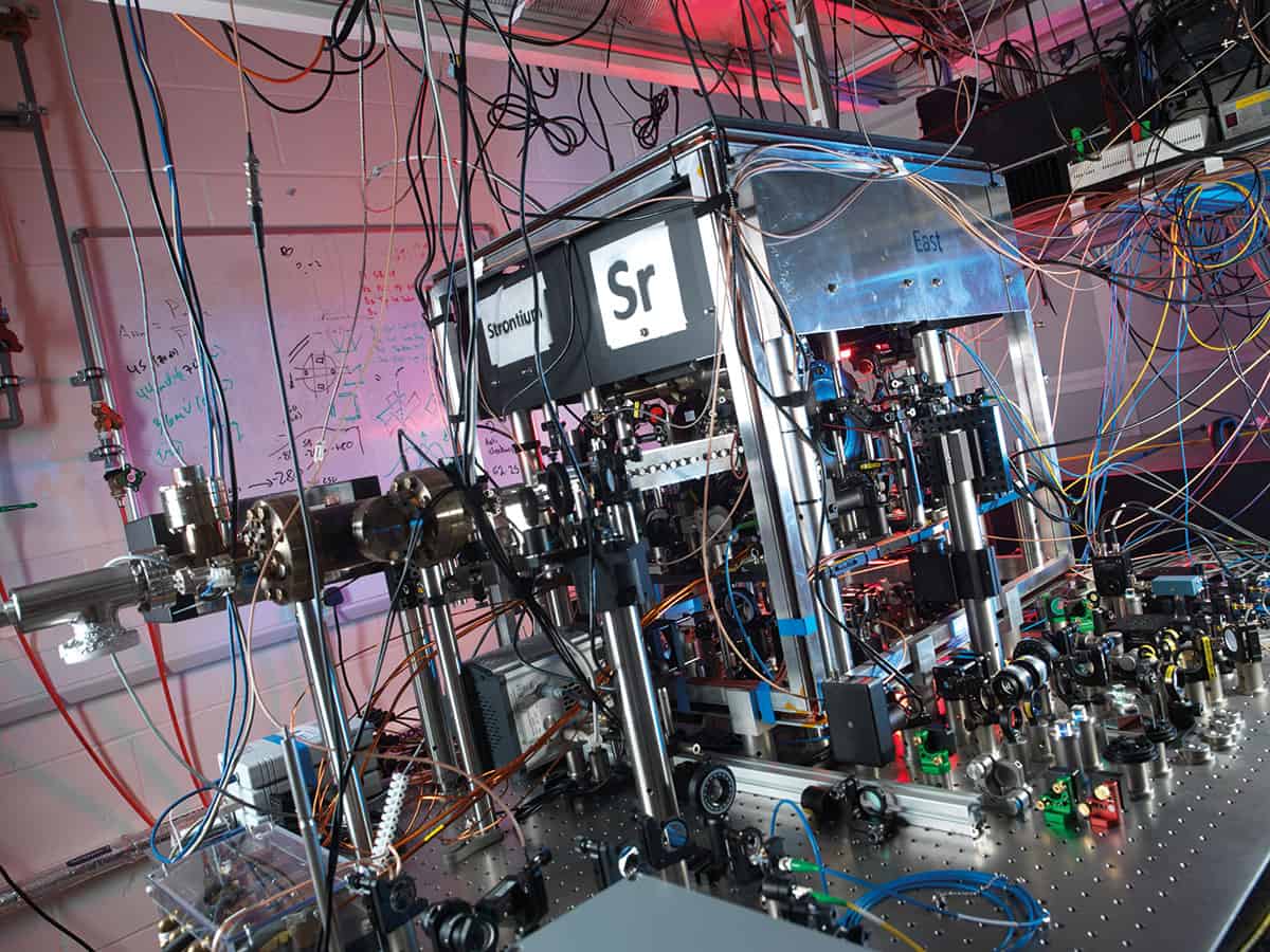
In an optical atomic clock, an ultra-stable laser is locked to a spectrally narrow electronic transition in the optical region of the spectrum – the so-called “clock transition”. The optical clocks being studied today fall into two categories: some are based on single laser-cooled trapped ions and others are based on ensembles of laser-cooled atoms trapped in an optical lattice.
The former, a single laser-cooled ion in a radiofrequency electromagnetic trap, comes close to the spectroscopic ideal of an absorbing particle at rest in a perturbation-free environment. When cooled, it can be confined to a region of space with dimensions less than the wavelength of the clock laser light, which means Doppler broadening of the absorption feature is eliminated.
By controlling its residual motion to ensure it is tightly confined to the trap centre, other systematic frequency shifts can also be greatly suppressed. This type of clock therefore has the potential for very high accuracy. The drawback is that a single ion gives an absorption signal with low signal-to-noise ratio, which limits the clock stability that can be achieved.
Neutral atoms, on the other hand, can be trapped and cooled in large numbers, resulting in a signal with far better signal-to-noise ratio. Stability, for example, improves with the square root of the number of atoms, all else being equal. Researchers can now confine thousands of laser-cooled atoms in an optical lattice trap – most commonly a 1D array of potential wells formed by intersecting laser beams.
One might expect that the light beams used to trap the atoms would alter the frequency of the clock transition. However, this can be avoided by tuning the laser used to create the lattice to a “magic” wavelength at which the upper and lower levels of the clock transition shift by precisely the same amount – a solution first proposed in 2001 by Hidetoshi Katori, from the University of Tokyo in Japan.
The current record for optical clock stability is held by Andrew Ludlow’s group from the US’s National Institute for Standards and Technology in Boulder, Colorado. Their ytterbium optical lattice clock recently demonstrated a stability of one part in 1018 for averaging times of a few thousand seconds. However, trapped-ion optical clocks have also demonstrated stabilities well below those of caesium atomic clocks, and both types have now reached estimated systematic uncertainties at the low parts in 1018 level. This far surpasses the accuracy of caesium primary standards and raises an obvious question: is it time to redefine the second once again?
The future of time
The frequency of the selected optical standard would, of course, need to be accurately determined in terms of the caesium frequency, to avoid any discontinuity in the definition. But this can easily be accomplished using a femtosecond optical frequency comb – a laser source whose spectrum is a regularly spaced comb of frequencies – to bridge the gap between the optical and the microwave frequencies. One obstacle to a redefinition is that it is unclear which optical clock will ultimately be best. Each system being studied has advantages and disadvantages – some offer higher achievable stability, while others are highly immune to environmental perturbations.
Another challenge is to verify experimentally their estimated systematic uncertainties through direct comparisons between optical clocks developed independently in different laboratories. Here researchers in Europe have an advantage as it is already possible to compare optical clocks in the UK, France and Germany with the necessary level of accuracy using optical-fibre links. Unfortunately, these techniques cannot currently be used on intercontinental scales and alternative ways to link to optical clocks in the US and Japan must be found.
Remote clock-comparison experiments must also account for the gravitational redshift of the clock frequencies. For optical clocks with uncertainties of one part in 1018, this means the gravity potential at the clock sites must be known with an accuracy corresponding to about 1 cm in height, a significant improvement on the current state of the art. Tidal variations of the gravity potential must also be considered.
Although all these challenges are likely to be overcome given time, a redefinition of the second will require international consensus and is still some way off. Until then, the global time and frequency metrology community has agreed that optical atomic clocks can in principle contribute to international timescales as secondary representations of the second.
Indeed, the unprecedented precision of optical atomic clocks is already benefiting fundamental physics. For example, improved limits have been set on current-day time variation of the fine structure constant (α ≈ 1/137) and the proton-to-electron mass ratio by comparing the frequencies of different clocks over a period of several years.
Optical clocks could also open up completely new applications. By comparing the frequency of a transportable optical clock with a fixed reference clock, we will be able to measure gravity potential differences between well separated locations with high sensitivity, as well as high temporal and spatial resolution. Such measurements will lead to more consistent definitions of heights above sea level – currently different countries measure relative to different tide gauges, and sea level is not the same everywhere on Earth. They could also allow us to monitor changing sea levels in real time, tracking seasonal and long-term trends in ice-sheet masses and overall ocean-mass changes – data that provide critical input into models used to study and forecast the effects of climate change. It is ironic perhaps that we will be able to study the Earth – whose rotation originally defined the second – in greater detail with the help of its latest usurper: the optical clock.