Page 1109 – Physics World

Home » Page 1109

Loops and arcs in the radio sky

Over the last century, our understanding of the universe has changed dramatically. One key discovery we have made is that for the first 380,000 years, the universe was a hot opaque plasma of photons, electrons and protons. As the plasma expanded and cooled, the electrons and protons eventually joined to form hydrogen, for the first time creating a transparent universe through which photons could travel freely.

Those photons are still travelling to this day and are our evidence for this event in cosmic history. Our observations and precise measurements of these photons, known collectively as the cosmic microwave background (CMB), have played a key role in defining our modern view of cosmology. Not only does the CMB confirm the hot Big Bang model of the universe, but it also provides a portrait of the initial conditions that later evolved into the galaxies and galaxy clusters that we see today.

The photons of the CMB would originally have formed a hot black-body spectrum – the lopsided curve of intensity versus frequency that is characteristic of photons emitted at thermal equilibrium. However, in the billions of years since they were created, those photons have since been stretched, as the universe has expanded, to longer wavelengths to form a cold black-body spectrum with its peak at 160 GHz (equivalent to having just been emitted by a black body at a temperature of 2.7 K). However, the CMB is not the only source of radiation at these frequencies and so a big focus of CMB measurements is to avoid radiation from other sources, and – where this is not possible – to identify and remove it.

One source of contamination is the Earth’s atmosphere and man-made interference, prompting researchers to minimize this unwanted noise by carrying out satellite and balloon-borne experiments to obtain the most precise observations of the CMB. The European Space Agency’s Planck satellite is the latest such experiment, and it has provided us with the most precise full-sky maps of the CMB we have to date. Planck has delivered two sets of cosmology results so far, with one final set to come.

The most important result from the mission is that it confirmed that the cosmology of our universe is extremely well described by a model that has only six parameters – which Planck measured – with no evidence for any significant deviations. As a result, we now know the age of the universe with unprecedented precision to be 13.799 ± 0.038 Gyr; that the Hubble constant has a lower value than previously thought, of H₀ = 67.8 ± 0.9 km s⁻¹ Mpc⁻¹; and that ordinary (baryonic) matter makes up only 4.8 ± 0.1% of the universe, with dark matter accounting for 25.8 ± 0.5% and dark energy for the remaining 69.4 ± 1.2% (arXiv:1502.01582).

While the main driver behind the Planck mission was to make high-quality observations of the CMB, the telescope also unavoidably observed radiation from the whole of the rest of the universe as “foregrounds”. Planck observed the entire sky at nine different frequency windows from 30 to 857 GHz, in which radiation from different sources feature to a greater or lesser extent. By analysing and comparing these nine maps, researchers have identified the different radiation sources, or “components”, and cleanly subtracted them to accurately map the CMB. Identifying the components not only yields an accurate map of the CMB but also lets us learn a great deal about the interstellar medium of our Milky Way as well as nearby galaxies and distant galaxy clusters.

While the first Planck data release in 2013 provided information about the intensity of the measured radiation only, the latest 2015 data release also includes information on the radiation’s polarization – whether the electromagnetic waves oscillate preferentially along a particular direction, and if so, by how much. For the first time, also, the data have been decomposed into maps of all the different components, including several that contribute to the unwanted “foreground” (arXiv:1502.01588). (In the first release, in contrast, the different components that dominate in the three lowest-frequency maps were treated as a single foreground component.) Using Planck data we have recently studied these low-frequency maps, which are dominated by emission in the Milky Way, and revealed new and surprising features, both big and small, in the radio sky (arXiv:1506.06660).

The polarized sky

While the intensity of the CMB provides a snapshot of the universe at 380,000 years old, it is possible using another parameter of the CMB to examine the physical conditions of the universe at less than 10⁻³² seconds old. That parameter is the polarization of the measured electromagnetic waves. In some models known as “inflation”, in which the universe expanded by a factor of 10⁸⁰ in a fraction of a second after the Big Bang, gravitational waves are expected to have been created that may have produced a characteristic, detectable polarization field on the CMB. Detecting this pattern would confirm the inflationary paradigm and give insights into the extremely high energy scale of the early universe, which is why measuring the polarization of the CMB is so important.

In 2014 the BICEP2 team, observing the polarization of the CMB from the South Pole, controversially claimed to have detected a polarization pattern that would indicate the gravitational waves caused by inflation (2014 Phys. Rev. Lett. 112 241101). In response, the Planck team prioritized its initial analysis of the polarized sky and – together with the BICEP2 and Keck collaborations – published a joint analysis showing that the reported polarized signal was in fact mainly produced by polarized light emitted by dust in the Milky Way (2015 Phys. Rev. Lett. 114 101301). Whether there are gravitational waves from inflation at lower levels than BICEP2 and other current CMB experiments could detect is still unclear. Apart from more sensitive future CMB experiments, answering this question will also require us to characterize better the different sources of polarized light, be they from thermal dust, synchrotron emission or other processes entirely. That way we can avoid confusion about whether detected signals are indeed cosmological, or if they are simply from the Milky Way.

Oval-shaped (long-ways across the page) all-sky map in a rainbow and black colour scheme including cyan, purple, pink, red, yellow and green colours. A legend consists of the top half of a semicircle, which has radial coloured lines fading from cyan on the horizontal and going clockwise from left through purple, pink, red, yellow, green and back to cyan. The radius of this semicircle is marked as going from 0 at the centre to 50 at the edge, in units of brightness temperature (microkelvin). Most of the map is dark. The main feature is a cyan-coloured band that spans horizontally across the centre of the map; the feature is wider in some places, such as at the left edge where it is about a half of the height of the map, and narrower in others, such as across most of the middle where it it about an eighth of the height of the map. There are a few faint pink curves that cross the central horizontal vertically before curving towards the centre of the map. In the largest of these the pink curve transitions to yellow and green. A large dashed-white-line oval is overlaid on the map, which is tilted and spans over a third of the map wide and nearly the whole height of the map. Within this feature is a smaller dotted white line tracing most of a figure of eight, with the centre of the figure of eight being at the horizontal centre of the oval — **1 Synchrotron sky** This full-sky map shows polarized synchrotron emission at 30 GHz and was made using Planck and Wilkinson Microwave Anisotropy Probe data. Large coherent structures can be seen, which trace the magnetic field structure of the Milky Way. Loop I (dashed line) is one of the largest features in the sky. The Fermi bubble filaments are also shown (dotted lines). The colours indicate the angle of the projected magnetic field, which is derived from the measured polarization angles. The brightness represents the signal strength using a scale that highlights faint emission in the sky; for the majority of the scale range the colours are bright, but close to 0 µK they tend to black, which indicates no polarized radiation. Well-defined features of the same colour indicate that the magnetic field is coherent and aligned in that region. (Courtesy: Planck Collaboration)

To characterize the low-frequency polarized emission from the Milky Way (along with more distant foreground emission), Planck produced polarized maps of the sky at 30, 44 and 70 GHz (in addition to higher-frequency polarized maps at 100–353 GHz). These maps show synchrotron radiation generated by cosmic-ray electrons and positrons spiralling around magnetic field lines in the Milky Way at near the speed of light from almost everywhere in the sky. These polarized maps therefore give us information about the Milky Way’s magnetic field and the distribution of high-energy particles.

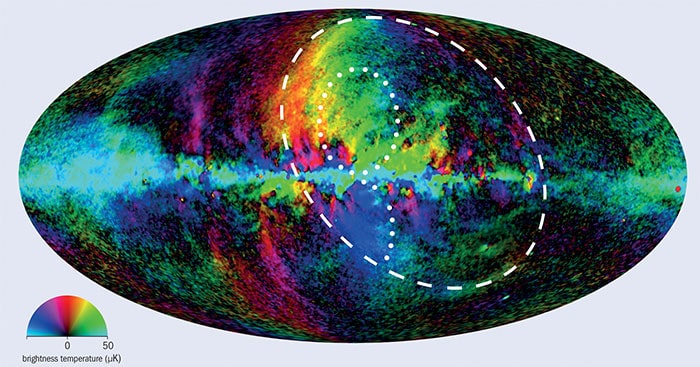
Figure 1 shows a polarized map of synchrotron emission that combines data from both Planck and NASA’s Wilkinson Microwave Anisotropy Probe (WMAP) at 20–50 GHz into a single map of the all-sky polarized emission scaled to 30 GHz. The hues indicate polarization angle, while the brightness of the colour represents the intensity of the polarized emission. The main feature is the plane of the Milky Way along the equatorial band of the map. The relatively uniform light blue along the plane tells us that the magnetic field is well ordered along our galaxy’s disc. A second striking feature is that most of the emission away from the galactic plane comes from individual filamentary structures, unlike the much smoother and broader structures seen in the intensity maps.

Some of these large-scale structures have been known since astronomers made the first radio surveys in the 1950s and 1960s, coining them radio “loops” and “spurs”. The sensitive Planck observations have given us new insights into the structure and properties of these features, with some thought to have originated from supernovae explosions, where an expanding shockwave compresses a magnetic field, accelerating electrons to relativistic speeds and producing radio emission. The large size of the loops (many times the size of the Moon in the sky) implies that the explosions occurred in the same part of the spiral arm of the Milky Way that the Sun is in – less than a few thousand light-years from Earth – causing them to appear large on the sky due to projection effects.

Much of the polarized emission in the sky is related to “Loop I”, the outline of which is shown in figure 1. This is one of the largest features in the sky – if you could see it with your eyes, it would cover the whole of the night sky. The loop’s ovoid shape has been fully traced for the first time with Planck data and its angular size on the sky is larger than what was originally thought. Its origin is probably connected to a number of supernovae explosions of high-mass stars within the last 20 million years that together formed what is known as a “superbubble”. It was long thought that these supernovae occurred in a region of young stars about 400 light-years away called the Scorpius-Centaurus Association. However, we have considered the radio polarization and X-ray intensity of the radiation coming from Loop I – quantities which both diminish as the radiation travels through interstellar gas – and we have found that there is not enough gas between us and the loop to account for the values we measure unless the distance to the centre of the loop is at least 1500 light-years from Earth.

Three oval maps are shown, stacked vertically and, from the top, labelled 30 GHz, 100 GHz and 857 GHz. The 30 and 100 GHz maps look very similar and consist of a finely mottled blue and orange pattern over all of them apart from the central horizontal of the maps, which are dominantly orange, with a faint thin white line going across the central part of the horizontal. The 30 GHz map has thicker orange and white bands than the 100 GHz map. The 857 GHz map looks very different in contrast. It is a fairly uniform reddish-orange, apart from a central horizontal band, which is white and swirly and spans about a third of the height of the map — **2 Out of obscurity** Full-sky maps made using the European Space Agency’s Planck satellite at 30, 100 and 857 GHz. The CMB can be seen as a noisy pattern at the top and bottom of the 30 GHz and 100 GHz maps, but at high frequencies (857 GHz) it is completely obscured by dust. The foreground emission present in the 100 GHz map, mostly along the galactic plane, is a combination of the dust emission seen in the 857 GHz map and the foreground emission in the 30 GHz map, which comes from free electrons scattering off positive ions, anomalous microwave emission and synchrotron emission. By using the foreground information from the 30 and 857 GHz maps, researchers can remove them from the intermediate frequency maps to produce a clean and accurate CMB map. (Courtesy: Planck Collaboration)

The Planck data have also let us analyse many fainter and smaller loops in other parts of the sky. Two other filaments might be connected to a much more energetic event. In 2010 the NASA-led Fermi satellite detected large bubbles – extending above and below the galactic centre – that emit gamma-rays. These “Fermi bubbles” are thought to be related to past jet activity from the supermassive black hole at the centre of the Milky Way. Planck data have shown that the two filaments are closely aligned with the edges of the bubbles – shown in figure 1 as dotted lines. These synchrotron filaments are thinner than Planck’s resolution, which confirms that the Fermi bubbles have very sharp edges and helps to constrain the models that describe how the bubbles could have been created.

Intensity foregrounds

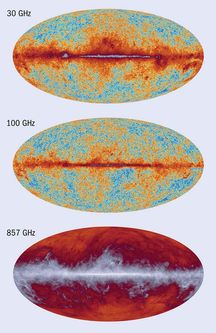
Although polarization data provide new insights into foregrounds, not every foreground component is polarized and we can learn a lot by looking at intensity alone. Figure 2 shows three maps that demonstrate the intensity foregrounds at different frequencies. At high frequencies (above 100 GHz) the foreground is mostly thermal emission from interstellar dust at temperatures around 15–25 K, as well as line emission from carbon monoxide and other molecules. At low frequencies (below 100 GHz) there is a mix of synchrotron emission from electrons spiralling around the Milky Way’s magnetic field, emission from free electrons scattering off positive ions known as “free-free emission”, and, unexpectedly, a dust-correlated component often referred to as “anomalous microwave emission” (AME).

AME is thought to arise from spinning dust particles that radiate as they rotate. It is typically found in photon-dominated regions where there are also lots of dust grains. Originally proposed by William Erickson in 1957, AME was largely forgotten about until it was discovered observationally in 1997 when CMB experiments started making sensitive measurements of the sky at around 30 GHz. Planck has given us the best evidence for AME in a wide variety of astronomical sources to date.

The complete set of Planck data provides new insights into all of these emission mechanisms. The fact that Planck observed at nine different frequencies means that all of these different emission mechanisms can be separated from each other using their spectral properties, in combination with data from WMAP and ground-based radio surveys.

Square-shaped image that is mostly black on the bottom half and purple on the top half, with a circular green feature in the centre that has a sliver of yellow on it's right side, and is encircled almost entirely by a pink border of uninform thickness. There are a few smaller yellow circular features elsewhere on the map — **3 Clear distinction** On this image of the Lambda Orionis region, red represents the anomalous microwave emission, green is emission from free electrons scattering off positive ions and blue is the synchrotron emission. The ring (pink) is around 200 light-years across, and surrounds the interior warm ionized gas (green). The yellow dots are background radio sources. The image spans 25 × 25 degrees of the sky; in comparison, the Moon’s angular diameter is a 50th of this image’s width. (Courtesy: Planck Collaboration)

A clear example where all three low-frequency components are spatially separated from each other, which was found for the first time by our recent analysis of the Planck data, is in the region of Lambda Orionis, shown in figure 3. The central region around the illuminating O8 star is dominated by free-free emission, but component separation reveals that there is a shell of AME surrounding the free-free emission, set against a background haze of synchrotron emission. This is the clearest example of an AME ring that has been seen, and it is one of only a few well-detected AME regions. The dust grains and molecules are irradiated by starlight in this photon-dominated region that lies at the transition between the warm ionized gas and the neutral interstellar medium. This illumination may be crucial for the dust grains to produce appreciable radio emission, either by electrically charging the grains, and/or by causing them to spin. More detailed follow-up observations are now needed to study the gas and dust in order to understand the physics behind the radio emission being produced by the dust in this region.

Looking ahead

The Planck satellite was switched off in 2013, but it has left us with a treasure-trove of data. Members of the Planck Collaboration are continuing to analyse the data, with the final set of papers due out in late 2016. The final version of the Planck data will also be released at the same time, and will be the best and most sensitive all-sky coverage until the next CMB satellite mission (possibly Cosmic Origins Explorer or Litebird) takes off, which may not be until some time in the next decade at the earliest.

Future experiments at different frequencies will help us further exploit Planck’s data. The C-Band All Sky Survey experiment, for example, will result in maps at 5 GHz that will let us characterize the synchrotron emission better, allowing an improved subtraction from Planck data and so yielding even better cosmological constraints. The next generation of CMB experiments – both ground-based and satellite – will provide us with better maps of the CMB polarization that will let us search for gravitational waves from the early universe, with the knowledge of the foreground emission provided by Planck being essential to clean up these maps.

Does the ‘softening’ of ice explain its slipperiness?

A new model of the slipperiness of ice suggests that a layer of disordered ice forms underneath a sliding object. The model was developed by Bo Persson of Forschungszentrum Jülich in Germany, and it could ultimately find practical application in helping to develop better skis, or improve traction in winter footwear or tyres.

Ice is, counterintuitively, not inherently slippery. Instead, it becomes so through the formation of a thin layer of meltwater on its surface. This liquid water can be created either by frictional heat or through a phase transition called premelting, which can occur at temperatures below the freezing point of water.

While premelting of ice surfaces has been studied extensively, the extent to which it plays a role in ice friction has long been unclear, explains Persson. Part of the challenge of investigating ice friction is that the interface between the ice and the object sliding across it is not easily accessible to molecular-level analytical techniques.

Shear stress

The core of Persson’s new study links a theoretical description of ice friction to existing experimental data. The outcome is a shear-stress law that can explain ice friction in terms of the sliding speed and temperature across a wide range of values. Sheer stress is the internal pressure in a material that occurs when that material is subjected to an external force along its surface. “To explain the measured data,” Persson says, “one must assume that the frictional shear stress in the area of real contact (which is very small compared with the apparent contact area because of surface roughness) decreases continuously towards zero as the temperature of the ice in the contact region approaches the bulk melting temperature.”

As the melting of ice is an abrupt phase transition, this decrease in friction with increasing sliding speed occurs more slowly than might be anticipated. Persson proposes two possible explanations. The first is that uneven frictional heating temporarily results in a nanometre-thick layer in which the ice is in a mixed state of adjacent, ice-like and water-like domains. Alternatively, a homogenous, heat-softened layer of disordered ice may form – and have a shear stress that decreases as the temperature increases up to the bulk melting temperature.

The latter, Persson says, is more likely, both given that heat softening is known to take place on the surface of ice, and that “the mathematical form of the frictional shear stress is consistent with what one may expect for premelting”.

Softening while sliding

Peter Sammonds and Ben Lishman of University College London and Dan Hatton of Plymouth University in the UK have collaborated on a previous study of ice friction, and they say that Persson “really adds something in pointing out that that lubrication is not the only factor, and that ice softening also plays a big part in the velocity-weakening friction regime”. They also point out that ice softening during sliding could possibly lead to larger contact areas between ice and slider when the slider stops moving. This in turn would affect the static friction between the ice and the slider, and lead to a memory effect in ice friction.

With this initial study complete, Persson is now moving to further refine his theory. To this end, he and his colleagues have constructed a sliding-friction instrument that can be cooled to –40 °C. This will allow them to incorporate a detailed measure of the impact on ice topography into the theoretical model.

At the same time, Persson is also conducting related work on rubber-on-ice friction, an area of study with particular relevance to the fabrication of winter tyres and the soles of shoes. In these cases, a different frictional process is likely to be dominant, Persson explains, one in which the surface roughness of the ice causes the rubber to deform, resulting in the dissipation of energy.

The research is described in The Journal of Chemical Physics.

Graphene-like boron made for the first time, claim researchers

The first boron films that are just one atom thick have been produced by a team of researchers at several institutes in the US. A preliminary study of the ultrathin material called “borophene” suggests that it displays a variety of fascinating and potentially useful properties including direction-dependent conductivity. However, unlike graphene – which comprises a single layer of carbon atoms – the boron films are not free-standing and are instead fixed to a metal substrate.

Since graphene was first isolated in 2004, physicists have been amazed at its extraordinary properties, ranging from extremely high conductance to extremely high mechanical strength. This “wonder material” has also inspired researchers to try to make free-standing, atomically thin films from other materials, and explore their properties.

Boron is one of the most fascinating elements in the periodic table: it is highly reactive, forming very strong and highly delocalized two- and three-centre bonds that are not truly ionic, covalent or metallic. Boron has 16 known bulk-crystal structures (or allotropes), but until recently there was no known 2D form. Predicting what such a structure might look like was difficult because unlike carbon, which forms 2D layers in graphite, boron has no layered allotrope.

Highly unstable

In 2007 Hui Tang and Sohrab Ismail-Beigi at Yale University proposed two possible 2D, free-standing monolayer structures comprising hexagonal bonding networks with periodic vacancies. Then in 2014 Lai-Sheng Wang of Brown University and colleagues discovered a nanoparticle comprising 36 boron atoms that could form a section of one of the sheets (called the α-sheet). However, in the same month, Artem Oganov and colleagues at Stony Brook University concluded that such a sheet would be highly unstable. Further progress was made last year when researchers in China found that a structure just two-atoms thick was produced when a mixture of boron and boron oxide was heated to 1100 °C and passed over a copper substrate.

Now, the Stony Brook team has joined forces with physicists at Argonne National Laboratory and Northwestern University to create and characterize two different – and previously unseen – boron structures that are both just one atom thick. They did this by depositing boron atoms onto a silver substrate at temperatures ranging from 450 to 700 °C. One structure is described as a metastable homogeneous phase and the other as a stable, corrugated “striped” phase. Northwestern’s Andrew Mannix explains that these two new structures are different from ultrathin boron films that have already been created by other teams. This is because previous films have been 2D analogues of 3D phases that are not really new structures.

You can create a whole new world of 2D borons
Artem Oganov, Stony Brook University

The team worked out the atomic structures of the new phases using various analytical techniques such as scanning tunnelling microscopy and electron diffraction. This involved joining forces with the Stony Brook group and using their structural-prediction algorithm to conclude that the stable striped phase should comprise a rectangular, corrugated lattice of boron atoms. This information was then used to calculate what scanning tunnelling micrographs and electron-diffraction data from such a structure would look like. The experimental data were consistent with these calculations, leading the researchers to conclude that their predicted structure is indeed correct.

Stiffer than graphene

By combining its limited experimental data with theory, the team predicts that the structure could have some interesting properties. These include electrical conductivity that depends on the direction of current flow. The material appears to be a metal along the direction of the stripes, whereas it shows evidence of a semiconductor-like band gap for current flowing across the stripes. A similar anisotropy is predicted in mechanical properties, with the material being twice as stiff (and stiffer than graphene) along the stripes as it is across the stripes.

The films studied by the team remained fixed to the silver substrate and a key question is whether or not the monolayer structure can be made free-standing. Oganov is sceptical: “Miracles do happen, and maybe free-standing boron will be one of them, but I have doubts.” He adds: “[Not being free-standing] is a clear disadvantage, but it also brings very clear advantages: graphene is graphene whether you put in on one surface or another surface. But by choosing the appropriate substrate you can tune the electronic state of 2D boron…You can create a whole new world of 2D borons.”

No vacancies

Lai-Sheng Wang is impressed. “I think these are certainly very credible results,” he says. “I don’t really see a weakness.” He adds, however, that “For an isolated monolayer, the most stable structure is with hexagonal vacancies. There is no hexagonal vacancy in these structures but I think that with appropriate conditions that may be formed.”

Indeed, in September 2015 Boris Yakobson and colleagues at Rice University in Texas predicted that a structure containing such vacancies would form on silver. Working independently, Kehui Wu and colleagues at the Institute of Physics in Beijing now claim, in a preprint on arXiv, to have detected Yakobson’s structure experimentally.

The research is published in Science.

Name the element, continued

By Michael Banks

It will soon be time to get the Tipp-Ex out on your copy of the periodic table.

That is because the International Union of Pure and Applied Chemistry (IUPAC) and the International Union of Pure and Applied Physics (IUPAP) have announced the discovery of four new elements: 113, 115, 117 and 118 – completing the table’s seventh row.

(more…)

The Soviet side of space

When the Apollo 11 astronaut Buzz Aldrin visited the Cosmonauts exhibition at the Science Museum in London, he was characteristically blunt, describing it as the story of a “competitor that lost”. Visitors without a direct link to the space race, however, will probably draw very different conclusions from this exhibit and its associated book. Cosmonauts is not so much a story of winners and losers as an incredible tale of what happened when humans left the planet for the first time.

The first steps of Aldrin and his Apollo comrades on the lunar surface marked a pivotal moment in the space race, but Cosmonauts reminds us that the Soviets had their own string of era-defining achievements. These included the first spacecraft to enter orbit (Sputnik, 1957) and reach the Moon (Luna 2, 1959); the first man and woman in space (Yuri Gagarin in 1961, Valentina Tereshkova in 1963); and the first spacewalk (Alexei Leonov, 1965). Chief among the marvels on display here is Tereshkova’s 2.6 tonne Vostok-6 descent module. It is sometimes possible to look at museum artefacts dispassionately, with a slight historical disconnect, but there is nothing abstract about the charred surface of this humble brown sphere: it really did leave our planet and come hurtling back at 27,000 kilometres per hour.

In contrast, the largest item in the Cosmonauts collection – a 3 tonne, 5 m-tall engineering model of the LK-3 lunar lander – remained firmly on the ground. After the death of chief engineer Sergei Korolev in 1966, the Soviet space programme lost its way somewhat, and the LK-3 never put a cosmonaut on the Moon. Still, it looks impressive, with a spherical body and spindly legs that resemble those of a giant metallic insect. It also had to be officially declassified before appearing in the exhibition, as it had previously been kept out of public view at the Moscow Aviation Institute. In fact, the entire crewed lunar programme had been kept secret until 1989.

Photo of visitors with an engineering model of the LK-3 lunar lander — **The almost Moon** Visitors with an engineering model of the LK-3 lunar lander, which would have carried a crewed mission to the Moon. (Courtesy: Science Museum)

Some of the most fascinating objects in Cosmonauts are the smaller accessories and the stories behind them, such as the first drawing in space (sketched by Leonov on Voskhod 2). Other insights into the cosmonauts’ experience come from the tools meant to help them survive after their descent modules crashed back to Earth: a standard survival kit included both a needle and thread (for repairing clothes) and a pistol (for shooting predatory animals). And an ejector seat used on the earliest Soviet flights, which carried dogs rather than humans, has a certain macabre humour to it: its plastic pooch looks hesitantly out of a plastic bubble hat.

Emma Smith, a member of the curator team, describes Cosmonauts as the most ambitious exhibition the Science Museum has ever undertaken. Part of the reason is that all but two of 150 artefacts were borrowed from Russia, with many coming from closed military enterprises and private collectors. In assembling the collection, the curatorial team made copious trips to Moscow and worked closely with their exhibition partner the State Museum and Exhibition Center (ROSIZO) as well as the British Council and the UK embassy in Moscow.

As well as persuading Russians to part temporarily with their invaluable cultural heritage, the other big challenge was to transport these large heavy objects to the UK without breaking them. In the case of Vostok 6 the challenge became even harder when asbestos was discovered in the heat-proof shielding – a substance forbidden for UK imports. Smith and her team managed to secure an exemption from the UK Health and Safety Executive on the condition that it was transported securely in a sealed environment. She recalls with fondness a training exercise when her team took a giant beach ball – purchased from a leading UK supermarket – wrapped it in cling film and practiced manoeuvring it around the exhibition space. Every little practice helps.

Vostok 6 and several other larger objects were too large to be flown so were transported in 20 m-long trucks by an armed security escort by road across the Finnish border, then by ferry from Helsinki to the UK. “I was quite nervous when we were crossing the Russia–Finland border because it’s quite an unusual object to be transporting,” says Smith. Upon arriving in London, the adventure was far from over as the exhibition is located on the first floor of the museum. Specialists were called in to lift the objects using hoists and gantries and Russian engineers were flown in to help with the reassembly of the LK-3 model.

Photo of a dog ejector seat and suit as used on suborbital rocket flights — **Space hound** Curator Emma Smith looks at a dog ejector seat and suit as used on suborbital rocket flights c. 1960. (Courtesy: Science Museum)

Cosmonauts also explores Russia’s cultural fascination with space travel. This stretches back to the late 18th century, when the “cosmist” philosophers argued that humanity’s destiny lay in space – the only place that could set us free from the imperfect realities of life on Earth. Later, in the Soviet era, the cultural connection was strengthened by the humble origins of many cosmonauts: both Gagarin and Tereshkova were from rural areas and had parents who worked as labourers. This helps to explain why ordinary citizens felt such a strong link with the missions. A lovely illustration of this is a letter written by a schoolgirl, Maria Kartseva, to Moscow Radio Committee in 1959. In it, she expresses her desire to fly to the Moon in her “warm skiing jacket, felt boots and a warm fur hat”.

Ultimately this is a universal story, and to argue that Cosmonauts makes a case for a Soviet space “victory” is to limit your appreciation of this fine exhibition. It’s a thrilling journey, this business of stepping into the infinite blackness. Why not enjoy the ride?

Cosmonauts: Birth of the Space Age
Science Museum, London
Exhibition runs until 13 March 2016
Scala Arts Publishers £45.00/$75.00hb 256pp

A version of this article appeared in the December 2015 issue of Physics World.

The January 2016 issue of Physics World is now out

Polarized patterns: the cosmic microwave background as you’ve never seen it before. (Courtesy: Planck Collaboration)

By Matin Durrani

Happy new year and welcome back to Physics World after the Christmas break.

It’s always great to get a new year off to good start, so why not tuck into the first issue of Physics World magazine of 2016, which is now out online and through the Physics World app.

Our cover feature this month lets you find out all about the Planck mission’s new map of the cosmic microwave background. Written by members of the Planck collaboration, the feature explains how it provides information on not just the intensity of the radiation, but also by how much – and in which direction – it’s polarized.

(more…)

Fabiola Gianotti takes charge at CERN as lab weighs up designs for future colliders

This is a month of change at the CERN particle-physics lab near Geneva with the Italian physicist and former ATLAS spokesperson Fabiola Gianotti becoming the15th director-general of the lab since it was founded in 1953. On 1 January she succeeded Rolf-Dieter Heuer, who has stepped down after seven years in charge to take up a place on a new seven-member panel that will provide scientific advice to the European Commission.

Gianotti was chosen to succeed Heuer in late 2014 and spent last year shadowing her German predecessor to get prepared for the role. “My priority as CERN director-general will be to expand and maintain CERN’s excellence in four areas: science; technology and innovation; education; and peaceful collaboration,” Gianotti told physicsworld.com.

To help her accomplish these goals, in late 2015 she announced three new CERN directors, whose appointments were quickly approved by the lab’s council that is run by its 21 member states. They also took the reins of the lab on 1 January. Gianotti’s fresh management team is made up of four other CERN directors. The quartet includes the particle physicist Eckhard Elsen, who was formerly at the University of Hamburg and the DESY lab in Hamburg. He is the new director for research and computing, taking over from the Italian physicist Sergio Bertolucci, who had held the position since 2009.

Change at the top

Gianotti has also changed the structure of the directorate to introduce two new roles. Previously, CERN had a director for administration and general infrastructure – a position held by Sigurd Lettow. This position has now been split into two. Martin Steinacher, a former chair of CERN’s finance committee, will become the lab’s director for finance and human resources, while Charlotte Warakaulle, former head of the United Nations Library in Switzerland, will be CERN’s director for international relations.

Meanwhile, the CERN council also approved the re-appointment of Frédérick Bordry as director for accelerators and technology. He has been at the lab since 1986 and has been director of accelerators and technology since 2014 when he replaced Lyn Evans. “We have made some changes in the organizational structure”, says Gianotti. “But it is no big revolution.”

Targeting high luminosity

During his five-year term, Elsen will be in charge of the entire scientific programme carried out at CERN. Elsen has extensive experience in particle physics, having worked on a range of experiments such as JADE and H1 at DESY, OPAL at CERN, as well as DELCO and BaBar at the SLAC National Accelerator Laboratory in the US. Until 2014 he was also chairman of the Large Hadron Collider Committee (LHCC), which plans, discusses and reviews the entire research programme carried out at the LHC.

“If new physics is there we can discover it, but it is in the hands of nature” Fabiola Gianotti, CERN director-general

Elsen told physicsworld.com that one of his first priorities will be to see what comes out of the LHC’s “Run II”, which began last year and will continue until 2018. It has routinely achieved collision energies of 13 TeV – almost double that reached during the LHC’s first run, when the Higgs boson was discovered. LHC physicists are hoping that Run II will not only lead to a better understanding of the Higgs mechanism, but also could throw up new particles and physics beyond the Standard Model. “My aim for the year is to do our best to deliver and collect high-quality data from the 13 TeV run,” says Gianotti. “If new physics is there we can discover it, but it is in the hands of nature.”

The LHC was originally designed for collisions at 14 TeV, rather than the current maximum of 13 TeV, and running at the higher energy will require the magnets being “trained” for that energy. However, Gianotti admits that running at 14 TeV is not at the top of her to-do list. “We will have to see how the magnets react to training for higher energies,” she says. “We will evaluate later on whether to go to 14 TeV or not.” Elsen highlights the LHC’s high-luminosity upgrade, dubbed “HL-LHC“, as another of the lab’s priorities for the new directorate.

HL-LHC will have a beam luminosity 10 times that of the current LHC and will require upgrades to the collider’s injection system to ensure the beam quality is good and stable enough. Improvements must also be made to the LHC’s main detectors – ATLAS, CMS, ALICE and LHCb – to handle the increased number of events.

Plans in place

Elsen says that CERN is “near to completing how to fund” HL-LHC, adding that it would cost around €500m for ATLAS and CMS, while the price tag for the other experiments will be around €60m. Bordry agrees with Elsen that HL-LHC is a big priority for the lab. “We now have all the plans,” he says. “So we have to implement it.” CERN’s directors are also interested in what will come beyond the LHC. Bordry highlights two studies, both led by CERN, for future particle colliders that would replace the LHC. “The role of director is a strategy role,” says Bordry. “My role is to prepare the future of CERN and particle physics.”

One design is the Compact Linear Collider (CLIC), which would smash electrons and positrons together at 3 TeV. Unlike protons – which are made of quarks – electrons and positrons are fundamental particles and this means that their collisions produce far fewer unwanted particles. As a result, such a collider could be used to make high-precision measurements of the Higgs as well as other particles that the LHC may find in the future. Construction of CLIC could begin in the 2030s when the LHC shuts down.

The other collider is a much more ambitious circular proton–proton machine that could run at 100 TeV to search for new particles. Such a collider would have a circumference of 80–100 km, making it much larger than the 27 km LHC. Yet Bordry is keeping his options open in terms of developing novel technologies. “We also have to look at how plasmas could be used to drive a proton beam,” he says.

Mathematical impressions

Between the early spring of 2008, when he began working on Landau damping and the Boltzmann equation, and the summer of 2010, when he won a coveted Fields Medal for that work, the mathematician Cédric Villani was a very busy man. That much is clear from Birth of a Theorem, Villani’s personal and highly idiosyncratic account of this crucial period in his career. It is worth stating up front that this book breaks essentially all the rules of popular science and maths writing: whole pages of it are filled with equations and LaTeX notation that even most mathematicians won’t follow, while technical terms usually go undefined and famous colleagues pop in and out like lights on a firefly.

But Villani isn’t trying to explain his work; he’s trying to explain what it was like to do that work, and in this he succeeds brilliantly. The book is, essentially, an Impressionist portrait of a mathematician’s working life, and reading it is a mixture of zooming in to examine the brushstrokes and backing away to get the bigger picture. There is no single moment where everything clicks together, but it’s an immensely rewarding read, and it does, eventually, give readers a very good impression of what Villani’s Fields-Medal-winning work was all about, and why it matters.

Farrar, Straus and Giroux £18.99/$26.00hb 272pp

Climate hopes, climate dreams

Photo of the Great Barrier Reef, with lots of colourful fish, corals and other sea life — Reasons to be cheerful: Although the Great Barrier Reef is almost certainly doomed, Tim Flannery finds room for optimism in his new book about climate science. (Courtesy: iStock/Michael Leidel)

For a book with the word “hope” in the title, the latest work from the Australian climate scientist Tim Flannery certainly gets off to a depressing start. Atmosphere of Hope was written in the run-up to the climate summit in December 2015, when world leaders met in Paris to hash out a plan for reducing carbon emissions enough to limit global warming to 2 °C (a target that was later revised, optimistically, to 1.5 °C). But as the opening chapters of the book make clear, a planet that is “only” 2 °C warmer is not exactly a utopia. Both wild habitats and marginal crop-growing regions are expected to suffer at the 2 °C mark, while a mere 1.5 °C rise above pre-industrial average temperatures (which some experts regard as inevitable despite the Paris agreement)would be enough to damage most of the ocean’s coral reefs beyond recovery. “It fills me with despair to admit it, but my beloved Great Barrier Reef is doomed,” Flannery writes sadly.

But within this generally pessimistic picture, he argues that there are still reasons to be cheerful. Falling demand for coal, he notes, has hit prices in Australia and other major exporters, making it more likely that this dirty fuel will remain in the ground. Better still, he writes, there are signs that “some of the same mice that are eating away at coal’s future have entered the oil business”. The main reason for Flannery’s optimism, however, is what he calls “third-way technologies”: biological and chemical processes that could be harnessed to withdraw huge amounts of carbon dioxide (CO₂) from the atmosphere. Most of them – from seaweed farms to a silicate mineral called olivine that naturally absorbs CO₂ – are still at the demonstration stage, with more research required before they can be turned into large-scale projects.

As usual, the devil will be in the details, and in Atmosphere of Hope most of the really fine details are relegated to the footnotes. But with the outcomes of political negotiations uncertain, and geoengineering a minefield of unintended consequences, it is hard to argue with Flannery’s view that such technologies represent our best hope for avoiding a catastrophic degree of warming. The real question is whether the size of the solutions will match the magnitude of the problems – and at the moment, neither Flannery nor anyone else knows the answer.

2015 Penguin £7.99pb 288pp

A folding challenge

By Louise Mayor

Here at Physics World HQ we have seen a lot of origami cropping up in physics over the last few years, be it curved-crease origami, origami robots or even sheets of graphene oxide going for a stroll.

It seems that a growing number of physicists have cottoned on to the fact that origami – and the related art of kirigami, where cuts are allowed – can be very interesting from a physics point of view, with properties that can lead to novel applications over a range of length scales. If you are a member of the Institute of Physics, you can read all about it in “Flat-pack physics”, a feature by science writer Simon Perks published in this month’s edition of Physics World.

As part of some background research for this feature I came across some great origami designs. One in particular – a snowflake – caught my eye and I got in touch with its designer Dennis Walker, who has been a paper folder for about 35 years. Walker very kindly agreed to update his instructions for making the snowflake especially for Physics World. They are now nice and clear and you can find Walker’s updated pattern here (PDF).

As an origami novice I can attest that the pattern is possible to follow albeit challenging (one of my attempts is shown in the photo above). In following the instructions it will help to know that dashed lines represent “valley” folds, where the paper is folded upwards into a “V” shape with a crease at the bottom; and the lines containing alternate dots and dashes represent “mountain” folds, where the crease is at the top and the paper is folded downwards into a “Λ” shape.

To start with you will need a piece of paper in the shape of a hexagon; you can find out how to cut a hexagonal piece of paper here. If you get stuck, do post a comment below describing exactly where you have got to. It may be that I or someone else can chime in to help you become unstuck.

What have snowflakes got to do with physics? Well, I am a physicist who just happens to enjoy puzzles and crafts, and I had a hunch that some of you might enjoy attempting this origami pattern too. But if I had to justify the link then I would point to Caltech physicist Kenneth Libbrecht’s classic Physics World feature “The enigmatic snowflake”, in which he describes the complex physics that governs how ice crystals grow, as he discovered by growing beautiful snowflake specimens in his lab.

Browse articles by content type

Loops and arcs in the radio sky

The polarized sky

Intensity foregrounds

Looking ahead