“Tilted table”, “peacock” and “triple-floor building” are just three of many fantastical 3D structures that have been created by compressing simple 2D patterns. The new technique for creating these objects is called compressive buckling, and has been developed by researchers in the US, China and South Korea. The method can be used to create objects with features as small as 100 nm that the team says could be useful for developing new technologies for medicine, energy storage and even brain-like electronic networks.
The ability to produce precision 3D structures on the micrometre or nanometre scale is becoming increasingly important to those developing a range of new technologies. However, the number of techniques currently available is limited. One option is to extend existing methods of manufacturing 2D (or extremely thin 3D) nanoscale structures such as computer chips to allow the creation of true 3D objects. This has proved to be difficult and time-consuming because it involves creating a series of aligned 2D layers on top of one another. Other techniques such as 3D printing, in which fluid nozzles deposit the required shape, lack precision and can be used only for materials that can be deposited as inks.
Silicon challenge
“They are highly constrained in the materials,” explains John Rogers of the University of Illinois at Urbana-Champaign, who is part of the compressive-buckling development team. “You can’t do it with silicon, for example, so there goes all of electronics,” he adds.
One alternative is to make a 2D shape and then apply mechanical forces to transform it into 3D. An established technique called “residual stress-induced bending” uses the stress between layers of two different materials on a 2D surface to cause etched objects to rotate out of the plane. This has been used to tilt micro-mirrors away from a surface, for example.
Now, Rogers and colleagues from the University of Illinois at Urbana-Champaign, Northwestern University, Zhejiang University, East China University of Science and Technology and Hanyang University have created a new 2D-to-3D fabrication technique. The first step is to use computer models to design 2D shapes that, when compressed at specific points held fixed to a surface, will relieve the applied compressive stress by buckling into desired 2D structures. The next step is to etch these 2D precursor shapes onto a silicon wafer and then chemically modify the points that must stay fixed when compressed. The pattern is then transferred onto a sheet of stretched silicone rubber. When the silicone rubber relaxes to its natural shape, the silicon precursor is compressed. The points on the silicon that had been chemically modified form chemical bonds to the silicone rubber and stay fixed, while the other points buckle upwards.
Creating design tools
Using this type of controlled buckling, the team managed to produce a variety of elaborate 3D shapes. The researchers even produced structures with multiple levels of elevation by designing shapes in which the relief of stress in the initial 2D shape would create further buckling, raising another part of the shape further. “We have senior co-authors on this paper who have developed really quantitatively precise models of how the mechanics works,” says Rogers. “We are just beginning to explore those models as design tools to investigate what range of topologies we can access in this way.”
Vladimir Aksyuk of the National Institute of Standards and Technology in Boulder, Colorado, commends the work. “This is interesting because it shows that, without having a built-in bilayer or residual stress gradient, you can go from purely planar to a diversity of shapes. That’s somewhat surprising to me,” he says. Vladimir Tsukruk of the Georgia Institute of Technology agrees, describing the variety of shapes demonstrated as “amazing” and the prospective applications of the technique as “astounding in breadth and impact”. This, he says, will be one of the key future challenges: to demonstrate that the technique can genuinely be used to make something that cannot be produced using a method currently in use or do it much more simply than before.
The team is now focusing its attention on these areas. Rogers looks forward to “an electronic cell or tissue scaffold”. “A lot of the people that we talk to are enthusiastic about what you can do when you go from a passive scaffold to something that embeds full electronic functionality,” he says. Rogers claims that this would allow researchers to produce “high-performance electronic networks in configurations that resemble the 3D networks that exist in the brain or the vasculature that provides blood flow to the heart”.
The first issue of Physics World magazine of 2015 is now out online and through our app.
As I outline in the video above, this issue looks at the challenges of synthesizing artificial human voices. Another feature explores the little-known Jesuits who boosted astronomy in China in the 17th century. And don’t miss our exclusive interviews with Fabiola Gianotti, who takes over from Rolf-Dieter Heuer as director-general of the CERN particle-physics lab early next year, and with Mark Levinson, the former physicist who directed the film Particle Fever about what particle physicists get up to.
We also have a fascinating feature about how you can help in understanding cosmic rays simply using your mobile phone. While most “citizen-science” projects involve people analysing data collected by “real” scientists, two new apps will let you collect data using your phone itself. Indeed, the people behind one of the apps think we’d need just 825,000 phones to gather as much data as are obtained using the Pierre Auger Observatory in Argentina.
Two physicists in the UK have added further insight into the seemingly paradoxical “quantum-pigeonhole effect”, which says that if three quantum particles are distributed over two locations, certain measurements will reveal that there is just one particle in each location. Alastair Rae and Ted Forgan of the University of Birmingham have calculated that quantum-interference effects can make it appear that each location only holds one particle, even though two particles might actually be present. They warn, however, that measuring the effect in the lab would be an extraordinarily difficult task.
The quantum-pigeonhole effect was introduced last year by Yakir Aharonov and Jeff Tollaksen of Chapman University in the US, together with colleagues in Italy and the UK. It is an extension of the classical pigeonhole principle, which simply says that if n objects are placed in n – 1 different locations (or pigeonholes) at least one location will contain more than one object. The team argued that in quantum physics, making a special sequence of measurements on three quantum particles that had passed through the equivalent of two pigeonholes would apparently reveal that no two particles had been in the same pigeonhole (see “Paradoxical pigeons are the latest quantum conundrum”).
Electron deflections
Tollaksen and colleagues had also proposed an experiment to verify this apparent violation of the pigeonhole principle. It would involve sending three electrons through a Mach–Zehnder interferometer, which contains a beamsplitter that creates two separate paths for the electrons. The three electrons are then brought together at a second beamsplitter before diverging to two different detectors (see the figure below).
Diagram of a Mach-Zehnder interferometer
As there are only two possible paths, you would expect at least two (and sometimes three) electrons to share a path. These two (or three) electrons travelling together would then be close enough to repel each other, deflecting their trajectories slightly. When all three electrons are detected, these tiny deflections should give a pattern of electron arrivals at the detectors that would reveal that two or more electrons had travelled along the same arm of the interferometer.
Tollaksen and colleagues focused on what would happen if the experiment were run in a certain way that involves only looking at the output of the detector – a process called “post-selection”. Under these conditions, they concluded, an experimentalist would not be able to tell that two electrons had travelled along the same arm.
Possible paths
Rae and Forgan have now analysed the outcome of such a hypothetical experiment, and have shown that applying quantum mechanics and the classical pigeonhole principle can explain the apparent paradox. Their calculations involve constructing the quantum-mechanical wavefunction of the three electrons in terms of the possible paths that the electrons can take through the experiment – all three electrons going through one arm, for example, or two electrons going through one arm and one through the other.
They find that if there is a relatively strong interaction between the electrons, you would see 12 spatially separated peaks at the detector, which would be a sign of the classical pigeon principle at work (see figure at the top of the article). In other words, there would be four peaks for each electron, corresponding to the four possible histories of the electron motion: travelling alone, with one or other of the other two electrons, or with both. If the interaction strength were zero, on the other hand, then only three peaks – one for each electron – would be measured in the detector. As expected, such a measurement will yield no information about how many electrons travelled through each arm of the interferometer.
Fooled by interference
Rae told physicsworld.com that things become very interesting when the interaction strength is small but finite. Three peaks would then be seen at the detector, and the pattern resulting from the interference between the four components of the wavefunction (all of which obey the classical pigeonhole principle) will look very similar to that which occurs when the interaction is zero. As a result, the observer might be forgiven for concluding that two or more interacting electrons had travelled through the interferometer without interacting.
Rae and Forgan also looked at whether it would be possible to run the experiment with electrons in the low-interaction-strength regime. Their calculations suggest that for 40 keV electrons, an experimentalist would have to discern patterns in their detectors across distances of about 10–13 m. This is about 1000 times smaller than the distance between atoms in a solid, making the measurement extraordinarily difficult if not impossible, according to the researchers.
“We used to look up at the sky and wonder at our place in the stars. Now we just look down and worry about our place in the dirt.” This lament from the main character in Interstellar, a semi-retired NASA pilot, carries a distinctly dystopian vibe and, indeed, the prospects for humankind at the outset of the film are dire. Set sometime in the not-too-far future (director Christopher Nolan never divulges an exact date), Interstellar depicts an Earth wracked with famine and plagued by a shortage of technological resources. Humanity’s only hope, it seems, lies with a motley crew of scientists and astronauts who must find a new home for what is left of the human race.
At its heart, Interstellar is classic space-travel science-fiction, and Nolan – an acclaimed filmmaker whose previous hits include Memento and the Dark Knight trilogy – tips his hat to a number of stalwarts in the genre, from Metropolis to 2001: a Space Odyssey, Blade Runner and even Avatar. But this is no chrome-clad futuristic world. Instead, human civilization has returned to an agrarian society, with a population that struggles to feed itself amid conditions that closely mimic the “Dust Bowl” of America’s heartland in the 1930s.
After a somewhat drawn-out beginning, the film picks up pace when an enigmatic NASA physicist (played by Michael Caine) reveals a plan to save humanity by jumping ship. But before he can figure out how to get the Earth’s entire population into space, through a conveniently placed wormhole and onto an alien planet in another galaxy, he must find out which of the 12 -planets on the other side of the wormhole is best suited for human habitation. With this in mind, NASA sends astronauts to assess the -planets’ potentials. When positive signals are received from three of them, a follow-up mission is organized in which Cooper, the aforementioned pilot-turned-unwilling-farmer, must manoeuvre a spacecraft and its crew of researchers through the wormhole to find out which planet best fits the bill.
With his easy Texan charm, actor Matthew McConaughey is perfectly cast as Cooper, the “space cowboy” who is also a father desperate to return to his children – especially his daughter, with whom he shares a special bond. Throughout the film, Nolan deftly combines the cold realities of interstellar travel with the messy business of human emotion, as Cooper agonizes not just about the success of their mission, but also about how long he has been away from Earth.
This is where the physics element of the film begins to shine through. Even with a handy wormhole at our disposal, interstellar travel is a lengthy business. The film is absolutely full to the brim with physics – not surprising, considering that the idea for it was born when a physicist, Kip Thorne, and a film producer, Lynda Obst, decided it would be fun to base a film on Thorne’s complex astrophysics research. The pair had previously collaborated on Contact, the 1997 film based on Carl Sagan’s novel, and after shopping their idea around Hollywood for several years it eventually ended up in the hands of Nolan and his scriptwriter brother Jonathan. Thorne remained heavily involved in the film’s development (he is an executive producer) and he has also published a book, The Science of Interstellar, to explain the physics that went into it.
The book was rushed into print in time for the film’s release and is a bit sloppily edited for my taste. From the perspective of your average cinema-goer though, a more serious flaw is that it reads like a cosmology textbook. While scientifically trained fans of Interstellar will gain much from it, others will be put off by the level of detail. Personally, I was initially thrown by its higgledy-piggledy order (the book does not follow the film’s timeline), but I did find Thorne’s system of labelling the book’s chapters with “T” for “truth”, “EG” for “educated guess” and “S” for “speculation” useful because it helped to distinguish established science from far-out guesswork.
The best part of the book, though, is the way that it shows how keen both Thorne and Nolan were to get the science right, and how the demands of the plot were matched to the rigours of reality. For example, at one point Nolan asked whether it was possible for one of the planets in the film to experience time dilation so extreme that one hour on its surface would translate into seven years on Earth. Thorne, for his part, did some serious research on what the astrophysical phenomena in the film would actually look like to nearby observers. He and a British visual-effects company, Double Negative, developed code to solve the equations that describe how light approaching a camera (or an eye) would misbehave in the vicinity of a spinning supermassive black hole.
In general, I had little issue with the science depicted in Interstellar. I did cringe slightly at its explanation of how, exactly, a wormhole was placed at such a convenient location, but (spoilers ahead) I found the idea of a four-dimensional “hypercube” lying deep within a black hole intriguing, and I could even suspend my disbelief about Cooper encoding complex data into the ticking of a wristwatch. As an avid science-fiction fan, I am reasonably happy to overlook a few stretched truths for the sake of a really good plot twist. But what distracted and annoyed me from very early on was the way Interstellar dealt with “habitable” planets. Data from NASA’s Kepler telescope indicates that there could be as many as 40 billion Earth-sized planets in the Milky Way, including 11 billion that may be orbiting Sun-like stars. Of these 11 billion possibilities, astronomers have already identified 47 Earth-like exoplanets that lie within the habitable zones of their stellar systems. None of them, however, are anywhere near a black hole. So why is it, then, that the five-dimensional time-travelling benevolent overlords in Interstellar – who can, after all, manipulate the laws of space–time to create wormholes, and who have a very good reason to care about the survival of humanity – choose new home planets for us in such an unappealing galactic neighbourhood? While I realize that the wormhole and black hole in Interstellar made the film exciting, surely they could have been incorporated in a way that did not make these god-like beings seem stupid, mean, or both.
Nolan wanted to make a science-fiction film that got the science right while also exploring the complex human issues around interstellar travel. On the whole, he succeeded. One could, perhaps, ask whether there is much point in having such complicated science depicted so accurately in a film, given that most viewers will be unable to tell (without reading Thorne’s book) what is and what isn’t fiction. However, after decades in which mainstream science-fiction films have happily flouted pretty much every known physical law, a film in which the science is, for a change, mainly true, can only be a good thing. Knowing that some directors make serious efforts to get the science right is, in itself, probably enough to inspire a few viewers – and perhaps even to push them to find out why a “black” hole can glow so brightly.
A little over a year ago, an eclectic group of (mostly) Australia-based researchers set themselves a challenge. On each day of 2014, they vowed, one of them would write a blog post about the crystal structure of an element, molecule or bulk material – one for every day of the United Nations International Year of Crystallography. As of early December 2014, they were tantalizingly close to completing their mission, with posts on more than 320 materials ranging from α-amylase (an enzyme in saliva that aids digestion of sugars) to zircon (a tough, diamond-like mineral found in some of the world’s oldest rocks).
Who is behind it?
The Crystallography365 website lists 33 authors, drawn from fields as diverse as chemistry, solid-state physics, structural biology and (of course) crystallography itself. Most are PhD students or early-career researchers, with a scattering of undergraduates and a few senior scientists who serve as “activators” in this scintillating mixture (see what we did there?). The project’s co-ordinator, Helen Maynard-Casely, works as an instrument scientist at the Bragg Institute in Sydney, Australia (named in honour of the pioneers of X-ray crystallography, William and Lawrence Bragg), and several other authors are likewise affiliated with its parent body, the Australian Nuclear Science and Technology Organisation (ANSTO).
What are some of the crystal structures that are covered?
The four crystals in the collection that begin with the letter “D” nicely illustrate its variety and, by extension, the importance of crystallography across many scientific fields. First up is diamond, one of three allotropes of carbon to get a blog entry of its own (buckminsterfullerene, graphite and tetrahedral amorphous carbon are the others). Next comes a mineral, diopside, whose structure was the first to be determined by studying how the intensity (rather than just the position) of peaks of diffracted light varies with the angle of incidence. The structure of the third “D” crystal, disulfide bond proteins, was discovered much more recently; these protein-folding enzymes help give structure to the walls of bacteria, and are thus a promising target for new antibacterial drugs. The final “D” in the collection is DNA, the subject of a blog post on 25 July – the birthday of Rosalind Franklin, whose X-ray crystallography images proved crucial to understanding the structure of this “molecule of life”.
Anything else of note?
The collection contains no fewer than 10 entries for water ice, from the hexagonal variety found in snowflakes (Ice Ih) to Ice XV. The latter substance, which was only discovered in 2009, is an ordered crystal that forms at low temperatures (below 150 K) and high pressures (around 1 GPa). There is also an entry for Ice IX – a real substance, but one that fortunately lacks the extraordinary properties attributed to it in Kurt Vonnegut’s science-fiction novel Cat’s Cradle (which was published 10 years before Ice IX’s real-life discovery). The emphasis on ice is partly Maynard-Casely’s doing: some of her previous research focused on the behaviour of ices under pressure, with particular applications to “ice giant” planets such as Uranus and Neptune.
Why should I visit?
Compared with some of its predecessors (particularly 2009’s International Year of Astronomy), the International Year of Crystallography received relatively little attention from the physics community – including, it must be said, in the pages of Physics World, which mentioned it only a handful of times. That’s a shame, because as Crystallography365 shows time and again, there is plenty of physics both in the techniques of crystallography and in what those techniques can reveal about the composition of the natural world. So, as physicists begin to celebrate the International Year of Light in 2015, it’s worth taking a moment to reflect on this one particular application of light and the riches of information it has yielded over the past century.
The arXiv preprint server received its millionth paper on 25 December 2014 – a major milestone for the repository, which was set up by the physicist Paul Ginsparg in 1991.
Cornell University’s arXiv has its roots in xxx.lanl.gov – a server set up by Ginsparg, who at the time was at the Los Alamos National Laboratory to share preprints in high-energy physics. It was originally intended for about 100 submissions per year, but rapidly grew in users and scope, receiving 400 submissions in its first half year.
The Indian government has given the go-ahead for a huge underground observatory that researchers hope will provide crucial insights into neutrino physics. Construction will now begin on the Rs15bn ($236m) Indian Neutrino Observatory (INO) at Pottipuram, which lies 110 km from the temple city of Madurai in the southern Indian state of Tamil Nadu. Madurai will also host a new Inter Institutional Centre for High Energy Physics that will be used to train scientists and carry out R&D for the new lab.
Originally planned to be complete by 2012, the INO has been in limbo for a number of years. In 2010 ecologists and conservationists raised objections to the INO’s initial proposed site at Singara in Tamil Nadu, which was near an elephant corridor and a tiger reserve. Researchers then had to find a new location, with the environment ministry only approving the Pottipuram site in 2011. Funding from the government arrived three years later.
The INO will be built some 1.3 km underground, accessible via a 2 km-long tunnel. The lab will comprise three caverns, the largest being 132 m long, 26 m wide and 30 m high, which will house a 50,000 tonne Iron Calorimeter (ICAL) neutrino detector. The detector will consist of alternate layers of some 30,000 “resistive plate chambers” and iron plates.
The outcome of this investment will be extraordinary and long term
Krishnaswamy Vijayraghavan, secretary of the Department of Science and Technology
The INO team hopes to use the detector to address the “neutrino-mass hierarchy”. Scientists know that there are three neutrino-mass states, but do not yet know which is the most massive and which is the lightest. “Understanding this will help scientists to pick the correct theory beyond the Standard Model and, along with other accelerator-based experiments worldwide, address the problem of matter–antimatter asymmetry in the universe,” says INO project director Naba Mondal, who is based at the Tata Institute of Fundamental Research in Mumbai (TIFR).
As well as housing other experiments such as those searching for dark matter and neutrino-less double-beta decay, scientists are also hopeful that the INO will provide opportunities for young students to work on all aspects of particle-physics research, such as detector development and data analysis. “Science students across the country will have the opportunity to participate in building sophisticated particle detectors and electronic data-acquisition systems from scratch,” says Mondal.
Indeed, Krishnaswamy Vijayraghavan, secretary of the Department of Science and Technology, which oversees funding for many science projects, says that the INO could “allow India to train experimental physicists and high-end engineers on a large scale” in “extremely important and competitive high-energy physics”. “INO will be the agent of transforming physics of this kind in India and will make a global impact,” he adds. “The outcome of this investment will be extraordinary and long term.”
Taking centre stage
Researchers also hope that the INO could help India to reclaim its leading position in neutrino physics and in constructing underground labs. The country led the way in the 1960s when physicists used a gold mine at Kolar in the southern state of Karnataka to create what was then the world’s deepest underground lab. Known as the Kolar Gold Field Lab, in 1965 it enabled researchers to detect neutrinos that are created when cosmic rays smash into the atmosphere. The lab later studied proton decay and was only shut down in 1992 when gold mining at the site became uneconomical.
“With the closure of the mines, we lost a unique facility for carrying out research in the field of non-accelerator-based particle physics,” rues Mondal. “With the approval of the INO facility, we are now back on the centre stage of particle-physics research.”
The family of chicken-sized birds native to South America called tinamous lay brightly coloured eggs that are some of the glossiest in nature. Now, an international team of scientists has discovered the secret to the eggs’ mirror-like sheen, which rivals that of highly polished man-made materials.
“Imagine a shiny, brand new car. The eggs of these birds are so shiny that they are reflective,” says Branislav Igic, an avian biologist from the University of Akron in Ohio, who did the work with colleagues in the US, the Czech Republic and New Zealand.
In the new study, Igic and his team used a combination of microscopy and chemical analyses to show that the glossiness of tinamou eggs is down not to pigments, but rather the nanostructure of the shell itself. In particular, the outermost layer of the shells, called the cuticle, is extremely smooth and composed of a unique mix of proteins and chemical elements such as calcium carbonate and calcium phosphate.
Smooth reflection
“A smooth surface means that light gets reflected back at the same angle that it comes in at,” says Igic. “A rough surface has tiny valleys and hills that scatter the light in all directions, and that leads to a more matt appearance.”
The study also reveals that the blue eggs of the great-tinamou bird are weakly iridescent – that is, the colour perceived by the viewer changes depending on the angle of observation and illumination. This optical effect, common in moth and butterfly wings, has never been seen in bird eggs before. “It’s a very subtle iridescence,” says Igic. “Human eyes may not be able to discern it, but birds have better colour acuity, so they are probably more sensitive to these changes in colour.”
Silvia Vignolini, a chemist at the University of Cambridge in the UK who studies colours in nature and who was not involved in the study, says the work sheds new light on how different bird species use combinations of materials and structural features to create various optical effects.
Surprising function
Mary Stoddard, an evolutionary biologist at Harvard University in the US who also did not participate in the research, says that the new findings reveal a surprising function for egg cuticles: “Typically, we think about the cuticle’s function in protecting the egg from bacteria or in containing surface pigment, but here the researchers show that it can also play an important role in producing the egg’s sheen.”
It is still unclear, however, why tinamous – and birds in general – lay conspicuous eggs that could make them more attractive to predators. In the case of tinamous, one important clue may be that it is the males and not the females who incubate the eggs.
Blackmailing males
“One idea”, says Igic, “is that by laying shiny, conspicuous eggs, females are blackmailing the males into incubating the eggs for longer periods, because otherwise the eggs would be easy targets for predators.”
Another possibility is that the eggs’ shininess is a by-product of a mechanism that reduces water exposure. “A polished surface might be better at repelling water, but this hypothesis hasn’t been tested yet so we don’t know for sure,” says Igic.
The research is described in the journal Interface.
As glaciers move faster, they experience less friction between the ice and the ground below. This is the conclusion of Lucas Zoet and Neal Iverson of Iowa State University in the US, who used a new experimental tool to simulate glacial sliding and demonstrate the importance of understanding how ice deforms to create cavities as it flows across large obstacles.
Given their potential for contributing to sea-level rise, understanding how glaciers move is vital to predicting their response to changing climates. However, gaining insights into how the underside of a huge piece of ice travels across the rough surface of the Earth is an extremely challenging problem. When modelling the flow of ice sheets, an increase in a glacier’s sliding speed was assumed to result in a corresponding increase in drag. In the late 1950s, however, the French glaciologist Louis Lliboutry proposed a more complicated sliding law – one in which increasing speed could ultimately result in a decrease in drag, once a threshold sliding speed has been exceeded. At the heart of this alternative theory is the impact of cavities that form in ice in the wake of obstacles on the Earth’s surface.
Bumps and pockets
“As ice slides forward, it has to viscously deform to get around a bump, much like water has to viscously deform to get around a stone at the bottom of a stream,” explains Zoet. Unlike with water, however, the ice is slow to fill in behind the obstacles that it passes around. “This leaves a pocket behind the bump of a size that is dependent on how fast the ice is sliding and how much pressure is acting on the ice to close the pocket,” Zoet adds.
As the glacier slides faster, the sizes of the cavities formed increase, extending out further behind the topographic obstacles that created them. According to Lliboutry’s theory, on an idealized glacier bed comprising a series of sinusoidal bumps, drag can be decreased when the cavities become large enough to extend beyond the inflection point of the next bump in the series. While this “double-value theory” has been the subject of debate, the difficulties of studying sub-glacial processes in the field – via boreholes, for example – have prevented it from being empirically tested.
To better explore these processes in a controlled setting, Zoet and Iverson created a new experimental device for simulating glacial sliding in the laboratory. Their simulator consists of a ring of ice 90 cm in diameter and 21 cm thick that is rotated above a rigid, sinusoidal bed. A hydraulic ram applies a constant downward force on the ice, simulating the weight of an overlying glacier while also allowing for the growth or contraction of cavities at the bed interface. The simulator operates within a cold room, with an additional fluid cooling system maintaining the ice ring at its pressure-melting temperature of 0.01 °C. Windows in the wall of the simulator allow the internal deformation of the ice to be observed, through the displacement of plastic marker beads embedded into the ice.
More realistic sliding rules
The researchers conducted a number of experiments to determine the relationship between the drag exerted on the ice and its sliding speed. “Lliboutry’s predictions matched our results well,” Zoet told physicsworld.com, adding that the results “will give theorists firm ground to stand on, moving forward, so that more complicated and realistic sliding rules can be developed”.
Ian Willis – a glaciologist at the University of Cambridge who was not involved in the study – calls the work “exceedingly valuable”, commenting that “it provides ammunition to the idea that existing large-scale numerical glacier and ice-sheet models – the sort of models that are used to project ice-mass responses to future warming – should incorporate such ‘double-valued’ sliding laws”.
Commending the design of the researchers’ experiment, glaciologist Martin Sharp of the University of Alberta agrees, adding that the double-valued relationship “could help to explain the episodic occurrence of ice avalanches, and the sudden changes in rates of glacier flow that are increasingly observed in the era of satellite monitoring of glacier velocities”.
The première was only 30 minutes away, and my voice was alarmingly hoarse. I had come down with a common cold just as I was supposed to play the role of the devious pilot Yang Sun in Bertolt Brecht’s The Good Person of Szechuan. Our enthusiastic amateur theatre group had been practising the piece three times a week for months, and I hated the prospect of having to cancel our first public performance. Luckily, one of the cast was a doctor, and she gave me a shot of industrial-grade cough medicine. Within minutes my voice had made a miraculous recovery, and I followed through with the 90-minute vocal ordeal.
The next day, however, I couldn’t utter a word – no sound whatsoever. My regular doctor instructed me to stay completely quiet for 10 days to let me heal my vocal folds – those twin flaps of mucous membrane in the larynx that vibrate to create sound when air is forced through them. My enforced silence caused surprisingly many inconveniences. The worst was that my wife couldn’t help thinking I was mad at her, despite knowing full well that I wasn’t giving her the “silent treatment”!
What this episode illustrates is that spoken language is simply such an integral part of our everyday experience that it is hard to imagine life without it. For me, my temporary lack of voice was a minor inconvenience, but sadly there are many people who are not able to speak at all. For some of them it is a disability they were born with, while others end up with no voice as a result of a stroke, an accident or cancer.
Although the spoken sounds we utter every day are effortless to produce, they are actually extremely complex
Fortunately, it is possible to help speech-impaired people with technological aids. And in this digital age we can do far better than the infamous bicycle horn of Harpo Marx. We can programme computers to turn text input into audio output, as evidenced by Stephen Hawking’s speech synthesizer. However, mimicking human speech is not as easy as it might seem. Although the spoken sounds we utter every day are effortless to produce, they are actually extremely complex. Communicating is not only a question of what you say but also a question of how you say it, and the how part is based on very subtle nuances.
It is these human-like how features that are very difficult to design into text-to-speech algorithms. In other words, it is hard to make computers speak with versatile and natural-sounding emotional content. Another problem is that it is tricky to synthesize a woman’s or a child’s voice – as these have a higher pitch than men’s voices – meaning that many women and children who have lost their voice have to use a speech synthesizer that sounds like a man.
Computer-generated speech
Designing and programming good speech-synthesis software is a daunting task. The most straightforward approach would be to record a huge collection of sample sounds, Each word would be read by a person at several pitches, with different emotional content – angry, loving, happy, strict and so on – and possibly for several dialects. Each word would need to be spoken by women, men, girls and boys, and for each language we wish to synthesize.
This method has its drawbacks, however. Consecutive samples do not necessarily fit well together, resulting in unnatural-sounding speech, while the processing power and computer memory required may make portable devices impractical.
An alternative approach, which is computationally more efficient, is to first analyse and understand speech by dividing it up into its structural components and then to synthesize each of these. This method, which Hawking uses, lets him control many aspects of speech, such as melody, rhythm and intonation, all of which are important in distinguishing statements from questions and for expressing emotion.
There are many mathematically and computationally challenging aspects of this method. In my research I focus on generating vowel sounds, which is hard but at least it suffices to model “static” sounds. Synthesizing consonants is even harder since it always involves dynamical, fast-changing features.
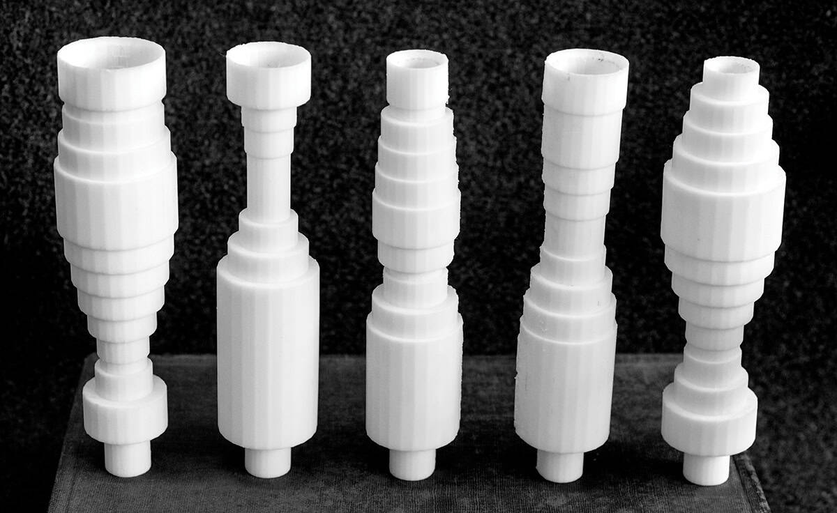
For model purposes These life-sized replicas of vocal-tract shapes were simulated on a computer to make the vowel sounds (from left to right) “a”, “i”, “u”, “e” and “o”. Produced by 3D printing in the Industrial Mathematics Laboratory of the University of Helsinki, these physical models, which accurately represent the computational models, are crude – the longitudinal axis of the real vocal tracts is curved instead of straight, and the cross-sections are not circular. Nevertheless, holding a vibrating electronic larynx to the end of these tubes demonstrates that these five shapes do provide decent vowel sounds. (Courtesy: Samuli Siltanen)
A vowel sound consists of two independent ingredients. The first is the sound produced by the vocal folds flapping against each other, known as the glottal excitation signal. (The vocal folds and the gap between them are called the glottis.) The second ingredient is the modification of this sound by the vocal tract, which is the curved and intricately formed air space between the vocal folds and the lips.
Let’s try a simple musical experiment to demonstrate. While the suggested performance may not hit the charts, it illustrates the independence of the two components of a vowel sound. First, sing “Mary had a little lamb” with all the words replaced by “love”. This shows that the same vowel can be uttered using an arbitrary pitch (well, within some limits, obviously). Second, sing the words “sweet love” at the same pitch as each other. This demonstrates how the pitch can be kept the same while singing two different vowels.
The pitch of a vowel sound is measured in hertz and is the number of times the glottis closes in a second. The vocal folds are actually the fastest-moving parts of the human body, with the pitch of a typical male voice being between 85 and 180 Hz, and that of a female voice from 165 to 255 Hz. The pitch of the vowel sound comes solely from the glottal excitation signal.
As the “sweet love” example above shows, even when two different vowel sounds have the same pitch it is very easy to distinguish between them. The same goes for notes of the same pitch played by different musical instruments – think of how easy it is to tell the difference between a piano and a saxophone playing the same note, for example.
This quality of the sound that makes it identifiable – often referred to as the character or “timbre” – is best studied in the frequency domain. The simplest sound, known as a pure tone, contains only one frequency. The glottal excitation signal contains all frequencies equal to or higher than the pitch of the signal. However, the shape of a vocal tract modifies this signal to create a complex tone, in which some of these frequencies are damped and others emphasized to create a unique sound.
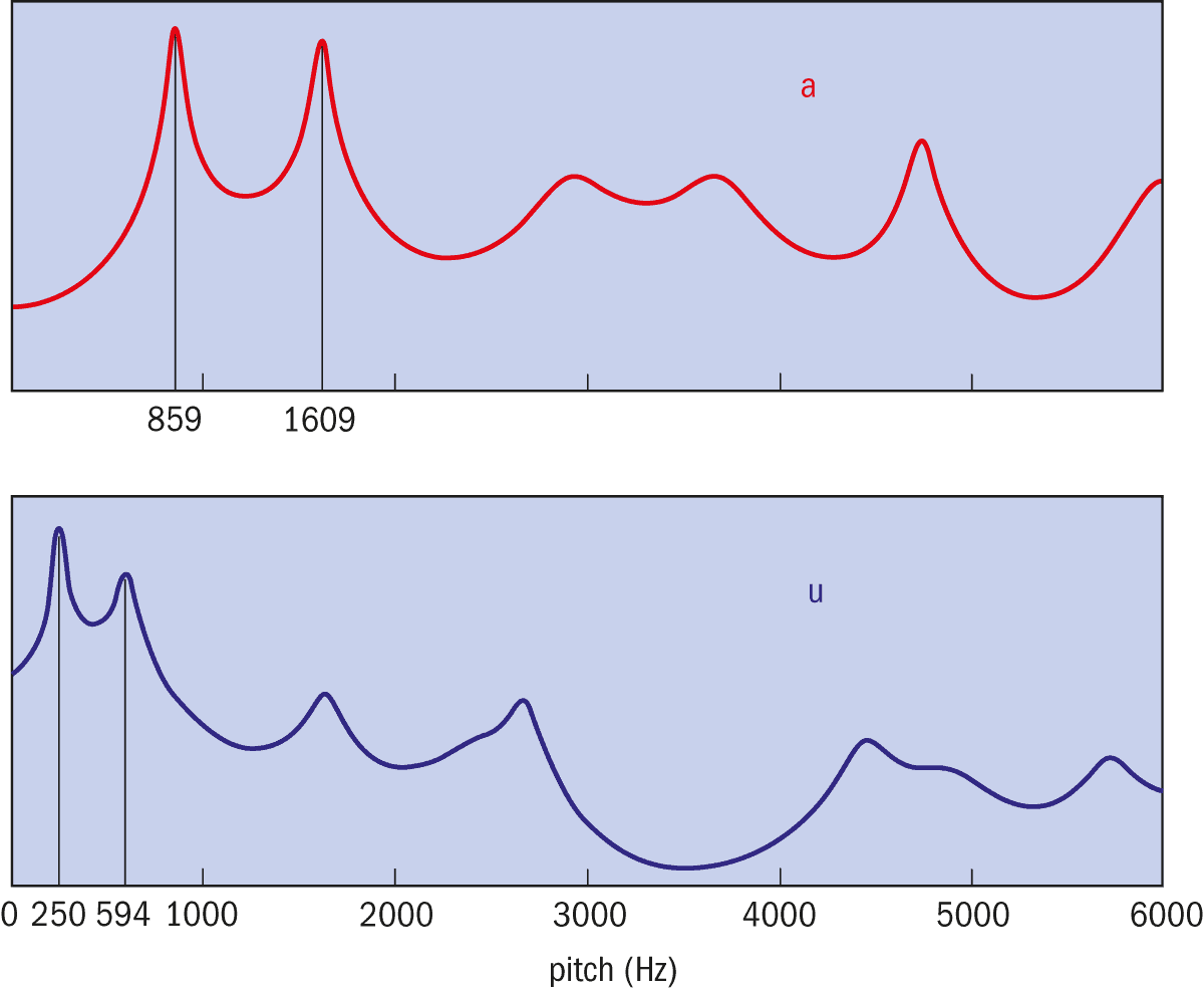
Figure 1
When people make vowel sounds, such as “a” in the word “car”, and “u” in the word “rule”, the effect of the vocal tract can be neatly observed in the so-called frequency domain. Similarly to a frequency equalizer on 1980s home stereos, the vocal tract emphasizes some frequencies and damps others. The most prominent frequencies are called the formants and define which vowel sound is being made. As shown here for example, the first and second formants for “a” are 859 Hz and 1609 Hz, while in “u” they are 250 Hz and 594 Hz.
Figure 1 shows examples of two vowel sounds in the frequency domain. Each vowel has two specific frequencies that are strongly emphasized, seen here as the two highest peaks: the so-called first and second formants. To make a particular vowel sound, muscles in the tongue, mouth, throat and larynx activate to give the vocal tract a particular shape in which these two formants resonate. You can observe a similar resonance when singing in a shower cubicle: certain notes seem to vibrate the whole bathroom, while others do not.
Creating natural-sounding vowels
To generate natural-sounding synthetic vowel sounds using a computer, we use a simple model for both the glottal excitation signal and the shape of the vocal tract. The excitation signal is described by a mathematical formula giving the amount of air flowing through the glottis at any given time (figure 2). Regarding the vocal tract shape, in the simulations we use circular tubes of varying radii, creating life-sized models of them for demonstration purposes (see the photo higher up this article). While these forms are far from the true anatomical shapes, they produce surprisingly natural vowel sounds.
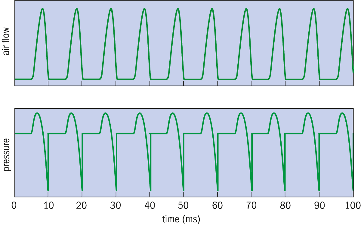
Figure 2
In our synthetic speech simulation at the University of Helsinki we simulate the periodic airflow through the glottis as a function of time, here with a pitch of 100 Hz (top). The vocal folds periodically flap against each other and every closure of the glottis brings the airflow abruptly to zero. Vital for our model is the pressure in the vocal tract as a function of time, known as the glottal excitation signal (bottom), which is calculated as the derivative of the airflow.
Good-quality synthetic speech needs natural samples of glottal excitations and shapes of vocal tracts. Those things are difficult to measure directly. The glottal excitation signal can be roughly recorded using a microphone attached to the Adam’s apple, and the shape of the vocal tract can be imaged using magnetic resonance imaging. It would be much nicer, however, if one could recover all that information simply from regular microphone recordings of vowel sounds. This in turn requires solving an inverse problem.
As with many inverse problems, the measurement data are not enough on their own to uniquely determine the cause
An inverse problem involves trying to recover a cause from a known effect. It is a bit like a doctor trying to find out the reason why a patient has joint pain, a cough and a fever: there are several different conditions that could lead to those symptoms. As with many inverse problems, the measurement data (i.e. the symptoms) are not enough on their own to uniquely determine the cause (i.e. the illness). Therefore, enough a priori information – such as ongoing epidemics, season and weather, the patient’s history of illness – has to be added in order to arrive at a correct solution. (A forward problem, incidentally, involves simply going from cause to effect: if the patient is known to be infected with an influenza virus, then the doctor can easily and reliably predict joint pain, a cough and a fever.)
A roulette of vowels
The inverse problem my collaborators and I are studying is called glottal inverse filtering (GIF). The starting point is a short vowel-sound recorded with a microphone and given to the computer in digital form. The aim of our method is for the computer to output a glottal excitation signal and a vocal tract shape that together produce as closely as possible the original vowel sound. The recovered excitation signal and vocal tract shape can then be used separately in many other combinations to produce a wide variety of different vowel sounds.
A simple trial-and-error approach would not work, as there are several different combinations of excitations and tract shapes that produce very closely the recorded vowel sound: in that case the effect is right but the cause, or structural components of the vowel, are wrong.
The GIF method we have developed is kind of a refined, probability-driven, trial-and-error procedure, which uses Bayesian inversion implemented as a so-called Markov chain Monte Carlo (MCMC) approach. As this gambling-related name implies, MCMC involves generating random values, which we like to think of as spinning a roulette wheel. (See the box below for more on this general method.)
For each vowel sound that we are trying to simulate, our MCMC-GIF method produces a long sequence of vowel sounds – typically 30,000 of them. The sequence is created using a random process subtly geared so that the average of all the 30,000 sounds in the sequence will be a nice solution to the inverse problem.
The gearing of the random process goes like this: the first sound in the sequence can be freely chosen. From then on, the next sound in the sequence is always defined either by accepting a candidate sound or rejecting the candidate and repeating the previous sound in the sequence. The candidate vowel sound is randomly picked by “spinning the roulette wheel”, or choosing a random glottal excitation signal and a random shape for the vocal tract. It is accepted only if it has high enough probability judged by the known measurement information (how close the candidate sound is to the original microphone recording) and the a priori knowledge (e.g. that the formants of the candidate are not too far from those of a typical vowel “a”).
Synthesizing speech by solving an inverse problem
In simulating speech using computers, we need to solve something called an inverse problem to produce natural-sounding vowels. This mathematical problem involves starting with a vowel sound and figuring out from it the initial conditions that led to that sound, i.e. the frequency at which the vocal tracts vibrated and the shape of the vocal tract.
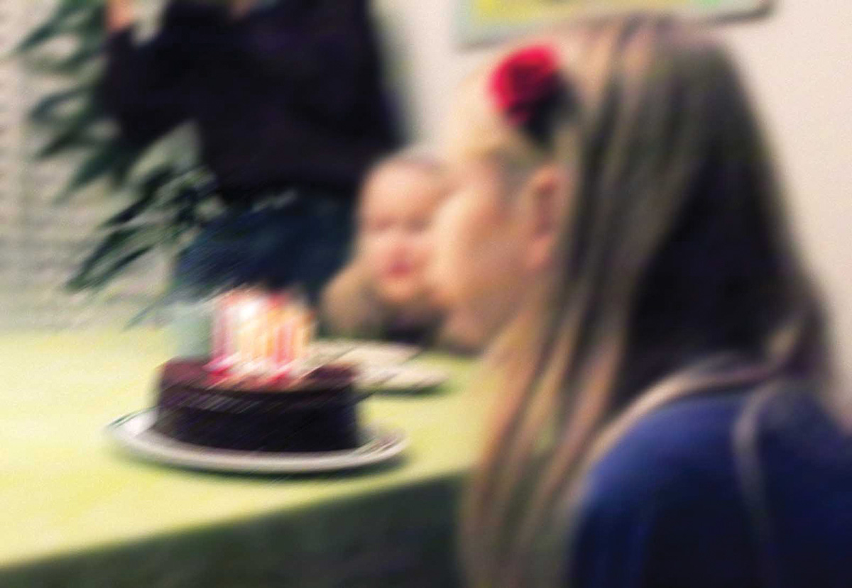
To illustrate how this method works, here is a simple example in which we estimate the age of an imaginary girl, Jill. Suppose we have a recently taken, badly focused photo of Jill blowing out the candles on her birthday cake. It seems that there are 10 candles, but we cannot say for sure. This is our noisy measurement information: the number of candles is 10, give or take a few. We can model the uncertainty using a Gaussian bell curve centred at 10 and having a standard deviation of, say, three years.
We also have a priori information: say we know Jill won a medal in the under 32 kg division of the last International Open Judo Championship. The historical record of medallists gives empirical probabilities: for example, there is a 4% chance that Jill is 9 years old and 13% chance that she is 11. Also, from the championship rules we know that she is definitely at least 8 and at most 15.
Let us now construct a sequence of numbers that are estimates of Jill’s age. The first number is 10 – the apparent number of candles on Jill’s birthday cake. To determine the next number we spin a hypothetical roulette wheel and call the result (a randomly picked number between zero and 36) the “candidate”. Now we either accept the candidate and add it to the end of our sequence, or reject it and instead repeat the last number in the sequence.
So how do we choose whether to accept or reject the candidate? What we do is to calculate the probability of the last number in the sequence and the probability of the candidate – the latter being the product of the photo-based probability (the Gaussian bell curve centred on 10) and the judo-based probability (given by the historical percentage). If the probability of the candidate is higher than the probability of the last number in the sequence, we accept the candidate. If the candidate is less probable, we do not reject it outright but rather give it one more chance. For example, if the probability of the candidate is a third of that of the last number in the sequence, we spin the roulette wheel again and accept the candidate only if the wheel gives a number smaller than or equal to 12 (which is a third of 36).
Finally, the average of the sequence of numbers generated with the above randomized method is an estimate for Jill’s age. The longer the sequence of numbers we generate, the better estimate we get.
Of course, in our simulation we’re not trying to compute an age but the frequency and vocal-tract shape that led to a certain vowel sound (see main text).
Voice of the future
Before our new method, there were no clear samples available of high-pitched excitation signals that women and children could use for natural-sounding synthetic speech. That’s because traditional methods are unable to solve the inverse problem for high-pitched voices – they cannot separate the excitation signal and the filtering effect of the vocal tract from each other. This means that the only option for many women and children is to use a speech synthesizer with a man’s voice.
In our work, we show that the probabilistic MCMC-GIF method can recover glottal excitation signals and vocal tract shapes more accurately than traditional GIF algorithms, even for voices with high pitch. Once these new computational advances are put in place, women and children will therefore be able to express themselves via computer-generated speech better suited to their identity. We hope that, as a result, quality of life will be improved for women and children who have lost their voice.
Our new method is still in the research phase in the sense that it is computationally quite expensive. However, now that we have demonstrated that it works, we are working on the next step – using mathematical techniques to speed it up. Once this is achieved we will be able to offer it to speech-synthesizer companies, who can then make the technology available.