The colliding of whipped-up grains of sand increases the strength of sandstorms, according to researchers from Brazil, China and Switzerland. Bouncing along above a moving bed of grains, collisions between particles in mid-air can propel them to greater heights – increasing the overall storm flux. These transport processes are vital to sandstorms and similar phenomena, which act to reshape a variety of geological landscapes.
Moving particles in a sandstorm can be grouped into three categories: creepers, leapers and saltons. Creepers are sand grains that remain at ground level, while both leapers and saltons are flung up into the air. The difference in the latter type of grain comes in the height that they can achieve. Saltons gain enough altitude that their impact velocity on landing – the so-called splash – sends other saltons up into the air. Together, these movements form saltation, the main aeolian or wind-based transport process.
Modelling flows
The role of mid-air collisions in such particle transport has long been debated, with the expectation that collisions between grains would cause particle movement to suffer an overall reduction. By creating 3D models of sandstorms, however – both with and without collisions – the researchers discovered that this is not, in fact, the case.
“Surprisingly, we found an enormous enhancement of mass transport by the wind in the presence of mid-air collisions, compared with the case when such collisions are switched off,” explains Nuno Araújo, one of the researchers at the Eidgenössische Technische Hochschule Zürich.
Counterintuitive findings
Unlike previous theories – which argued that saltons could only be formed during a splash – the team’s model revealed that leapers can become saltons through a series of mid-air collisions that gradually increase their altitude. The higher the particles go – as well as the longer they can stay in the air – the greater the acceleration from the wind, which increases the likelihood of saltation formation.
This was not the only counterintuitive finding. The team also observed that the storm flux – a measurement of strength based on the number of particles moving through a given area – actually increased when the sand particles were modelled to lose energy when colliding, compared with correspondingly simulated elastic collisions. This is because inelastic collisions acted to align the exit directions of the interacting grains – thereby increasing the flux in the direction of the wind.
The results of this simulation also help make it clear how sandstorms get going in the first place. As the wind grows stronger, grains are slowly dragged along the surface of the sand bed. “Because of irregularities in the surface profile, some particles will hop, eventually producing small splashes,” Araújo explains. Through this process, and with a high enough wind velocity, such splashes can create sufficient leapers to ultimately begin saltation. In fact, when the team modelled storms without mid-air collisions, all the aerial particles were seen to be leapers.
Whipping up a storm
Previous studies of interactions within sandstorms were hindered by having insufficient computing power to run such detailed collision models. Araújo and his colleagues were able to circumvent this issue by optimizing their simulation and using a logarithmic velocity profile to simplify the calculation of the turbulent air motion.
“[This] study gives us a fresh, physicist’s perspective on the concept of saltation – which is the key mechanism for the movement of sand,” comments Tom Gill, a geologist at the University of Texas-El Paso who was not involved in the study. “Since saltation is also the key to the genesis of dust storms, the new work could also improve the modelling and parameterization of the effect of dust aerosols on the global environment and climate system.”
“An interesting follow up would be to experimentally observe the role of mid-air collisions,” says Araújo. While it would not be possible to “switch off” collisions in real life, it would be possible to experimentally vary the restitution coefficient – the ratio of the relative velocities of the colliding particles – within certain limits. Other possible future work that the team proposes includes studies factoring in the aerodynamic lift of the particles, fluctuations in the turbulent wind speed or electrostatic interaction between the particles, or models that assess the role of saltation in different conditions, such as a terrestrial desert, submarine or Martian environment.
Running on hydrogen and oxygen and producing just electricity without any nasty emissions, fuel cells have over the years been used to power everything from bikes and buses to cars and even planes.
But last week saw the debut of a fuel cell at Imperial College London that was used to power a rock band. The fuel cell was unveiled at a summer barbeque organized by the Hydrogen and Fuel Cells (H2FC) Supergen Hub – a scheme funded by the UK’s research councils to boost interest in fuel cells among UK universities and businesses.
Researchers in Germany have succeeded in controlling tiny magnetic-spin patterns known as “skyrmions” for the first time. The result could be important for future high-density data-storage technologies and nanodigital electronic devices with improved data-transfer speeds and processing power.
Skyrmions are small magnetic vortices that occur in many materials, including manganese–silicide thin films (in which they were first discovered) and cobalt–iron–silicon. In the new work, the researchers studied a palladium–iron bilayer on an irridium-crystal surface. The tiny vortices can be imagined as 2D knots in which the magnetic moments rotate about 360° within a plane (see figure).
Skyrmions could form the basis of future hard-disk technologies. Today’s disks use magnetic domains (in which all of the magnetic spins are aligned in the same direction) to store information, but there are fundamental limits to the size such domains can be made. It might be possible to make skyrmions that are much smaller and that could therefore be used to create storage devices with much higher densities. What is more, flipping all of the spins in conventional domains – to switch a device’s memory state from 1 to 0, for example – requires considerable power and can be slow; skyrmions require fewer spin flips to switch. In addition, the final spin state is not easily disrupted – making these skyrmion structures more stable than conventional magnetic domains.
Creating and annihilating single skyrmions
Before skyrmions can be exploited in hard drives, however, scientists need to figure out a way to control them – something that has proved difficult to date. A team of researchers at the University of Hamburg, led by Kirsten von Bergmann, André Kubetzka and Roland Wiesendanger, has now shown that it is possible to create and annihilate single magnetic skyrmions using a spin-polarized current – one in which spin is mostly aligned in one direction – from a scanning tunnelling microscope (STM) tip, albeit at ultralow temperatures of 4.2 K. According to the researchers, the skyrmions switch from one state to another thanks to spin-transfer torques, and one state (skyrmions present) can be favoured over the other (skyrmions absent).
“To write or delete a skyrmion we position our STM tip at a particular spot on the sample and inject a spin-polarized tunnel-current pulse into it,” explains Von Bergmann. “While at low currents and voltages the sample magnetization is stable, at higher currents and voltages the magnetic state starts to switch between a skyrmion and a simple parallel alignment of magnetic moments,” she told physicsworld.com. “In this situation, the current direction can determine which of the states is favoured over the other – a clear indication that spin-transfer torque is involved in the switching process.”
IT applications
Being able to write and delete skyrmions in this way means that such spin textures can now be exploited in information technology. “In particular, the possibility of using layered thin films in this way, as is the case in conventional IT-device technology, could lead to a big step forward towards applications,” adds Von Bergmann.
The Hamburg team is now busy trying to understand the switching mechanism in more detail and finding out exactly how the spin-polarized current couples to the magnetization. “This will help us to optimize the process of writing and deleting skyrmions,” says Von Bergmann. “We will also be investigating other thin-film materials in an effort to unearth systems that show such skyrmion switching at room temperature.”
Skyrmions are named after the UK particle physicist Tony Skyrme, who in 1962 found that they could explain how subatomic particles such as neutrons and protons exist as discrete entities emerging from a continuous nuclear field.
The 2013 Dirac Medal has been awarded to three scientists whose wide-ranging work has brought profound advances in cosmology, astrophysics and fundamental physics. Thomas W B Kibble, Philip James E Peebles and Martin Rees all receive the honour, which is bestowed annually by the Abdus Salam International Centre for Theoretical Physics (ICTP) in Trieste, Italy. The three scientists will also each receive a prize of $5000.
Spontaneous symmetries
Thomas Kibble, emeritus professor at Imperial College London, has made major contributions to our understanding of spontaneous symmetry breaking – the process at the heart of the Higgs mechanism. Indeed, in an interview last year with Physics World, Peter Higgs named Kibble as one of at least five other theorists who deserve credit for predicting the existence of the Higgs boson. Kibble also explored the importance of symmetry breaking in a cosmological context – investigating what happens when a symmetry “disappears” as the universe evolves from the Big Bang.
“It is always very gratifying to have one’s work recognized by other physicists,” says Kibble. “This award is particularly special for me because of its association with my former colleague and inspiration, Abdus Salam, who founded the ICTP, and also because the other medallists this year are two astronomers for whose work I have the greatest respect – James Peebles and Martin Rees.”
Across the universe
Philip Peebles, a theoretical cosmologist who holds two emeritus-professor positions at Princeton University in the US, has worked on problems ranging from light-element synthesis to the nature of the dark universe. In the 1960s Peebles predicted some of the most important properties of the cosmic microwave background (CMB). He also quantified how galaxies cluster together to form large-scale structures over time and played a leading role in developing theories of “cold dark matter”.
At the heart of darkness
The third recipient, Martin Rees, is an emeritus professor at the University of Cambridge in the UK, where he has spent most of his research career. Like Peebles, Rees has also done pioneering work of the CMB and in 2005 the pair shared the $500,000 Crafoord Prize with James Gunn for their work on understanding the large-scale structure of the universe. Rees has a string of other achievements in astrophysics, including his work on the origin of quasars and the prediction that supermassive black holes lurk at the heart of galaxies.
In addition to his research achievements, Rees has also been instrumental in science policy and the democratization of scientific ideas, having authored several popular-science books. In 2011 Rees was awarded the £1m Templeton Prize for his “profound insights” into the nature of the cosmos that have “provoked vital questions that address mankind’s deepest hopes and fears”. He was also president of the Royal Society between 2005 and 2010, during which time he spoke to Physics World in this video interview about space, politics and scientific advice.
All three scientists received the prize today. Since 1985, the prize has been awarded annually on 8 August – the day on which the British Nobel-prize-winning theorist Paul Dirac was born in 1902. Dirac was a close friend of the ICTP, which was founded in 1964 by the Nobel laureate Abdus Salam as an international research centre to promote scientific excellence in the developing world.
“Our project concerned optimizing a manual longboard stand-up slide,” said Myles Cooper as he stood on a skateboard at the front of the class, holding an unattached skateboard wheel in his hands. It was the last day of “Advanced Classical Mechanics” (ACM), a course at Olin College in Massachusetts. Myles and two other first-year students, including my son Alex, were presenting their final project.
For non-skateboarders, Myles explained that a “longboard” is an elongated skateboard used for downhill cruising and tricks, “manual” means riding on the two back wheels only and “stand-up slide” means skidding, usually downhill. Longboarders consider slides to be awesome and have “slide jams” (see YouTube) to see who can achieve the longest slide without the wheels spinning. The group’s project was to use the tools of classical mechanics to find a function to optimize the distance that a rider could slide downhill on two wheels.
Was this an awesome diversion or effective pedagogy? I had come to Olin College to find out.
Exciting experiment
The college was conceived of in the 1990s as an ambitious response to repair the dismal state of US undergraduate engineering education. At that time, first-year engineering students came in passionate about their calling but half wound up ultimately changing their degree and a fifth dropped out of college entirely. The problem appeared to be an overemphasis on theory; imagine a music school that forced performance students to take three years of theory and harmony before touching an instrument.
In 1997 the F W Olin Foundation, set up in 1938 by the engineer-turned-businessman Franklin Olin, provided an initial $200m to create a new engineering college to foster students’ passion from day one. Most classes are organized around team projects. Olin’s founders call it “just-in-time” education – giving students the knowledge required to complete a project – versus “just-in-case” education, or loading students with knowledge for its own sake. The college is small, with about 350 students and nearly half of them female. The result is, in my view, the most exciting educational experiment in recent history.
As a parent of one of these students, am I biased? Totally. So don’t trust me, check the statistics. Some 98% of all Olin graduates get jobs or go to graduate school. More than 200 engineering programmes elsewhere have sent representatives to Olin to study the curriculum. Earlier this year three Olin founders, including the current president, Richard Miller, won a National Academy of Engineering prize for their efforts.
Though entranced by the educational concept, I was sceptical that physics could be taught effectively in the same project-based way as engineering. The ACM professor, Yevgeniya Zastavker, who has a PhD from the Massachusetts Institute of Technology, explained that ACM is less project-based than most courses at Olin College. Students do projects only at the end, although this work is integral to their education, providing them with hands-on application of physics to engineering contexts. She invited me to observe.
Complex affair
This is what Alex posted on Facebook the night before the presentation: “After spending 16 hours working in the same room save food breaks, spending two weeks figuring out how to model a two-wheeled longboard stand-up slide, running an extremely ridiculous set of differential equations for five days with no result, and possibly learning more about the physics of longboarding than probably any person ever, I AM FINALLY DONE WITH MY ACM FINAL PROJECT!”
A few hours after this post, the group members presented their work in class. They based their initial model on mass, acceleration caused by gravity, hill slope, angle θ between the slope and direction of wheel roll (θ= 0 follows the slope), and coefficients of static and kinetic friction. They created functions describing the system using these parameters for a given slope and θ, using MATLAB to plot these parameters. They found, for instance, that the longest slide with a slope of 15°, an initial velocity of 8 m/s and a constant θ occurred when θ was roughly 63°.
To maximize the slide path, however, requires constantly changing the value of θ. To analyse this further, the group first studied the energetics of the situation, using the Lagrangian approach to make three second-order differential equations for the relations of the system’s components in the x, y and z axes. They ran this through Maple (more powerful than MATLAB) but the presence of too many recursive functions made it impossible to solve. With their presentation looming they returned to a Newtonian approach in terms of forces, writing a MATLAB program that used equations from their first attempt but for which they had to keep resetting θ by hand. What seemed to be a simple system, in short, required complex analytic methods.
The same was true for the other groups that day. One modelled the forces on the college’s robotic sailboat. Another tried to model Spider-man’s iconic movement down a street by shooting silk strands at building walls – a series of spherical spring-pendulum motions in which he never hits the ground or walls. “It looks like a simple system to describe mathematically,” said Abe, a first-year student, “but it turns out that there’s not really an analytical solution and the system quickly becomes chaotic.”
The critical point
I came away convinced that much of classical mechanics can, indeed, be taught via the rigorous analysis of real-world situations “just in time”.
But not everyone appreciated the students’ work. The following complaint appeared on a Web forum on which Olin students had discussed skateboarding physics: “Why are you all trying to put square science into my fun hippie longboarding?” The students’ sarcastic response: “Don’t worry, we modelled the final trajectory with a quartic function, not a ‘square’ one!”
Accurate measurement of temperature is a key part of almost every science experiment, and in most cases, the measurement is relatively straightforward. However, with my colleagues Robin Underwood and Gavin Sutton at the National Physical Laboratory (NPL) in the UK, I have just spent six years measuring a single temperature – and we knew the answer before we started! Sort of.
Every measurement is a comparison of an unknown amount of a quantity with a standard amount of that quantity. But in most measurements this “comparison against a standard” is indirect and not immediately apparent to the user. For example, when a shopkeeper weighs out 500 g of grapes, neither they nor their customer are immediately aware of the calibration chain that stretches from the shop, via the local “weights and measures” laboratory, to NPL and on to the unique lump of metal in the vaults of the International Bureau of Weights and Measures (BIPM) in Paris that is our standard kilogram.
For temperature, the standard amount to which all other temperatures are compared is the temperature of the triple point of water, TTPW. To be sure, most people using a thermocouple to measure the temperature of an oven are not aware of this, but it is still true. If you were to visit NPL you would find a dewar filled with glass cells containing water held at its triple point, the temperature of which we use to directly calibrate thermometer readings.
At TTPW, liquid water, solid ice and water vapour co-exist in equilibrium and this is chosen as the standard temperature because it can be reproduced relatively easily with an uncertainty below 0.001 °C. Currently, TTPW is defined to be 273.16 K (or 0.01 °C) exactly. Scientists could have chosen any number to associate with this temperature, but this particular choice is made so that the magnitude of both a kelvin and a degree Celsius is close to the historical degree centigrade.
This definition has served us well for more than 50 years. But for many scientists – myself included – it is unsatisfactory. The reason that temperature is defined this way is a hangover from the fact that we learned to measure temperature before we understood what temperature was. If, 200 years ago, we had understood that temperature was a measure of the energy of atomic motion, we would have defined temperature directly in terms of energy. And that is what we now hope to do.
In statistical mechanics, temperature always occurs in combination with the Boltzmann constant, kB. Currently, because TTPW is defined exactly, if one measures the product kBTTPW then all the uncertainty in the product is expressed as an uncertainty in kB. We think this is irrational and that kB should be – as its name implies – a constant, and defined exactly.
In this conception the kelvin would be defined by kB, which – like the speed of light in vacuum – would have an exact value with no associated measurement uncertainty. Since the units of kB are joules per kelvin, this will relate temperature directly to energy, and link it firmly into the rest of the International System of Units (SI). In that way, in future, every temperature measurement will be fundamentally a measurement of the energy of atoms and molecules.
Our work is part of a wider effort to redefine the base units of the SI in terms of natural constants. The second and the metre are already defined in this way, and metrologists are busy worldwide trying to achieve the same goal for the kilogram, ampere and mole, an effort discussed in depth in Robert P Crease’s March 2011 article “Metrology in the balance”.
A sound approach
Our approach to measuring kBTTPW was to make life easy for ourselves and pick a physical system in which we could achieve the lowest possible uncertainty. Back in 2007 we thought hard about all the possibilities and chose to make a measurement of the speed of sound in a monatomic gas. There were two compelling reasons for this choice.
In future, every temperature measurement will be fundamentally a measurement of energy
First, the speed of sound in the limit of low pressure, c0, in a monatomic gas is directly related to the root-mean-square speed of molecules, vRMS, by the strikingly simple relationship c0 = √(5/9)vRMS. So if we could measure c0with low uncertainty, then, if we knew the mass of the molecules, m, we could directly estimate the average kinetic energy of molecules, ½mv2RMS. Statistical mechanics tells us that for a lowdensity molecular gas this is equal to 3 × ½kBT. For more detail on the equations, see “Pinning down the product”.
The other reason for choosing to measure the speed of sound in a monatomic gas is that it is possible to make amazingly precise measurements of this value. The most obvious method for doing so is to measure the time it takes for a sound wave to travel a fixed distance. The measurement becomes more accurate as one makes the distance longer but that makes knowing the temperature over the whole path very difficult. The “trick” is to use a resonator.
In this technique one “folds back” the sound path so that it bounces around inside a cavity. Normally the sound from each reflection interferes destructively with sound from the loudspeaker and the sound pressure level inside the resonator is low. However, if one picks a frequency at which multiples of the wavelength precisely match the dimensions of the resonator, then constructive interference – resonance – takes place. By measuring the frequencies at which this happens it is possible to deduce the speed of sound, knowing the dimensions of the resonator.
One of the main advantages of this technique is that the speed of sound can be found independently from several different resonances varying in frequency from about 2 to 20 kHz. So the extent to which they agree provides a powerful self-checking feature. The problem is that although frequencies can be measured very accurately, it is much more difficult to measure the dimensions of the resonator. And even more challenging, the dimensions will of course change with temperature and pressure. We therefore had to choose the shape of the resonator very carefully.
In our work at NPL, we have been using a resonator in the shape of a triaxial ellipsoid. It is almost perfectly spherical, except that its x-, y– and z-radii, each approximately 62 mm, differ from each other by ±0.05% (32 µm). It might seem strange that distorting a sphere could result in a better measurement, but it does. The reason is that we used microwave resonances to measure the resonator’s internal dimensions and – unlike acoustic resonances – microwave resonances are degenerate in a sphere. This does not mean that the resonances are lacking in moral character; it means instead that there are several resonances with the same frequency. The triaxial distortion we created “lifts” this degeneracy, allowing us to measure a single resonant frequency for each principal radius. Our ability to measure the x-, y– and z-radii with nanometre resolution at the same time as measuring the acoustic resonances means any thermal expansion of the resonator can be accounted for.
Finally, we cooled the experiment to TTPW. We knew the temperature was correct because we had previously calibrated six resistance thermometers in a cell containing water, ice and water vapour in equilibrium. We transferred these thermometers into our apparatus without disconnecting even a single wire in case this caused a spurious change in voltage that might be mistaken for a temperature change.
So our experiment worked like this. By measuring microwave resonant frequencies, we could estimate the size and shape of the resonator. Then, knowing the size and shape of the resonator, measurements of acoustic resonant frequencies allowed us to infer the speed of sound. We measured the speed of sound of seven resonances at different pressures and extrapolated to the limit of zero pressure (figure 1). This told us the limiting low-pressure speed of sound, c0, and from this we could infer the mean molecular speed and hence the mean molecular kinetic energy, and hence kBT. And finally, because we carried out the experiment at TTPW, which is currently defined exactly, we were able to deduce kB with low uncertainty.
1 Intercepting the speed of sound A crucial calculation in our experiment was that of the speed of sound at the limit of low pressure, c0, of the argon in our resonator at the temperature of the triple point of water. It is not possible to achieve zero pressure, i.e. a perfect vacuum, but extrapolating several measurements of the speed of sound (squared) over a range of pressures gave our answer.
This type of experiment – the results of which may affect the future assigned value of the Boltzmann constant – requires a very defensive approach. So we do not claim to have the right answer. What we are claiming is that we can prove that the right answer – whatever it is – cannot differ from our answer by more than our specified uncertainty. To make this claim stack up, we need to separate the final result into a number of sub-results and evaluate each of those in different ways and see if the answer changes. In this experiment there were three quite distinct parts: a measurement of how close we were to TTPW; a measurement of the molar mass of the argon we used; and a measurement of the speed of sound, which depended critically on the size and shape of the resonator.
Sadly, the features editor of Physics World flatly refuses to turn over this entire section of the magazine to a discussion of our experiment, so here are two highlights of the measurement, concerning our estimate of the radius of our resonator and our estimate of the speed of sound.
Precision engineering
In order to reach our target of measuring kB with an uncertainty below one part in 106, we needed to measure the average, a, of the resonator’s three radii with an uncertainty substantially less than 0.5 parts in 106, or roughly 31 nm, on a radius of 62 mm. This was – to put it mildly – challenging. So we chose to begin by making the resonator from two hemispheres, each manufactured with breathtaking precision.
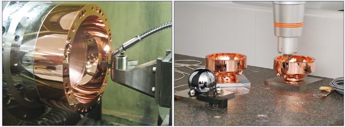
For this we enlisted the help of Paul Morantz and colleagues at Cranfield University in the UK, who are more used to sculpting mirrors for space telescopes. It took months to design the apparatus to simply hold the hemisphere on the lathe without straining the copper. Long experience had taught Morantz that to create two perfect quasi-spheres, we would need to start with eight “blank” hemispheres, and pick only the best candidates to make the final cut that defines the inner shape.
A triaxial ellipsoid has no rotational symmetry, and so to create such a shape on a lathe is a challenge. The angular rotation of a hemisphere must be measured in real time, and the single-crystal diamond-cutting tool moved back and forth in synch with the rotation (figure 2a). This involved adjusting the position and speed of the tool thousands of times a second by a program written in MATLAB. Morantz considered every aspect of the interaction of the diamond tool as it cleaved through the copper, and specified where the tool should be at every millisecond. The result of all this effort is an artefact of stunning beauty with a mirror finish with only nanometres of surface roughness.
2 Mirror perfection We collaborated with colleagues at Cranfield University who are expert at sculpting mirrors for space telescopes to create two “hemispheres”, which – when assembled – created a triaxially ellipsoidal cavity. The nominal radius was 62 mm and principal y– and z-radii differed from the x-radius by 32 μm. Carving a shape with no rotational symmetry using diamond-turning technology (left) is extremely challenging, but was achieved by programming the lathe to adjust the position of the tool thousands of times per second. To map the dimensions of the hemispheres, we used a co-ordinate measuring machine (right). To characterize the uncertainties involved in this measurement, we also mapped a silicon sphere that we knew the dimensions of from previous experiments.
The resulting four hemispheres were measured using a mapping instrument known as a co-ordinate measuring machine (CMM), and shown to be within 1.5 µm of their design shape over the entire surface. At the same time as we measured the hemispheres, we also made measurements on a highly perfect silicon sphere the size of which we already knew (figure 2b). In this way we could correct for errors in the CMM and we eventually achieved an uncertainty of measurement of 132 nm on the average radius. Not bad, but not good enough.
One difficulty was that to estimate the shape and size of the resonator when assembled, we had to take account of the fact that the flat surfaces of the hemispheres were only flat to within a wavelength of light – and so they did not quite mate perfectly. We also had to consider the changing shape of the hemispheres as we tightened the bolts to hold the hemispheres together.
To measure the average radius of two assembled hemispheres we used microwave resonances. This involved inserting two tiny wire antennas so that they were just flush with the inner surface. When the wavelengths of microwaves just fit inside the resonator, the transmission from one antenna to the other increases strongly. By measuring the frequencies at which these resonances occurred we could estimate the average radius in terms of the speed of light.
Crucially we did this with eight different resonances at frequencies from 2 to 20 GHz and the results agreed within a staggeringly tiny uncertainty of just ±3.5 nm. When one encounters this level of consistency in an experiment one has to concede that nature is trying to convey a message. Inserting acoustic transducers into the sphere – so we could measure the speed of sound – made the agreement between radius estimates from different microwave modes a little worse but our final uncertainty estimate was still only 11.7 nm. Which was good enough for us.
So because of all these checks, we feel confident in our estimate of the average radius because although we have tried, we cannot see any way that it could be wrong by more than about 11.7 nm.
Skinny sound peaks
The propagation of sound through a gas consists of a repeating cycle of exchange between thermal and mechanical energy. As the gas is compressed it becomes heated, and energy is stored as compression of the gas. As it expands, it cools and the thermal energy is transformed back to mechanical energy.
In the bulk of the gas this process is almost lossless, but for our estimate of the speed of sound we had to consider that within approximately 0.01 mm of a solid wall, the heat of compression is quickly “wicked” away, resulting in loss of energy in a so-called thermal boundary layer.
It took months to design the apparatus to simply hold the hemisphere on the lathe
For a monatomic gas, the speed of sound should not depend on frequency in the acoustic range. So using a resonator we were able to check our answer by working out the speed of sound from several different resonances over a wide range of frequencies. For each resonance the effect of the thermal boundary layer is different and so we had to apply an adjustment based on our theoretical understanding of the thermal boundary layer. Adjusting data makes us uncomfortable, but we are confident that we have done this correctly because estimates of c0 based on different resonances agreed with an uncertainty of only 0.09 parts in a million.
However, when we looked at the widths of our resonances, we were not pleased: we found that they were narrower than expected. In one extreme case a resonance with a frequency of 3548.8095 Hz was expected to be 2.864 Hz wide, but instead we found the width to be 2.858 Hz. We were flummoxed.
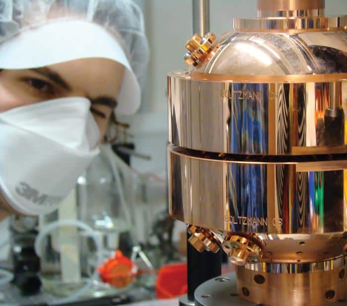
An eye for detail Robin Underwood assembles the resonator used to measure the Boltzmann constant. (Courtesy: Michael de Podesta/NPL)
When energy is lost as sound bounces around inside the resonator, the frequency profile of each resonance broadens. So having resonances that are too broad is understandable – it means there is a little bit of extra loss somewhere in the resonator. But having resonances that are too narrow meant there was something going on in the resonator that we did not understand. And since we were unaware of what this thing was, we could not easily assess how wrong it could make our answer.
However, after publishing the “line-narrowed” data at the 9th International Temperature Symposium in 2012, a colleague from the National Institute of Standards and Technology in the US, Keith Gillis, showed us the results of his new theory of a spherical resonator on which he had been working. His theory evaluates the effect of the thermal boundary layer to an additional level of precision. To our surprise and relief, his theory matched closely what we had observed. It was not that our resonances were too narrow, it was the theory that had not been sufficiently developed.
Making it official
In July Metrologia published our new estimate: kB= 1.380 651 56 (98) × 10–23 J K–1 where the (98) represents the uncertainty in the last two digits (Metrologia 50 354). The relative standard uncertainty is 0.71 × 10⁻⁶ , significantly less than our target of 1 × 10⁻⁶ , so personally, my work is done.
But NPL has not been working alone. Through 2014 we expect further estimates to be submitted to the Committee on Data for Science and Technology, which will consider their uncertainty estimates and relative consistency and come up with a recommended value and an uncertainty.
And then if the various committees and sub-committees of the BIPM agree, a proposal will be made by the International Committee on Weights and Measures to change the definition of the kelvin. If that is agreed by the General Conference on Weights and Measures when it meets in either 2014 or 2018, then the relative standard uncertainty of kB and TTPW will swap places: the value of kB will become exact and the value of TTPW will become uncertain. If the eventual uncertainty is close to 0.7 parts in 10, then the uncertainty in TTPW would become 0.19 mK.
You may at this point be wondering whether you will be affected by this change. Let me reassure you: you will not. I can be confident of this because almost everyone in the world measures temperature according to a procedure called the International Temperature Scale of 1990, which specifies how to practically calibrate thermometers, and for the moment, nothing in this procedure will change.
However, since 1990 we have discovered that temperatures estimated by this procedure (called T90) are slightly in error in that they differ from thermodynamic temperature – the familiar T in your equations of physics. The extent of this error is small by most people’s standards, with T–T90 growing from zero close to TTPW to about +4.5 mK at 29 °C and, –9 mK at –100 °C.
So having spent six years making the one temperature we thought we knew a little more uncertain, we have now begun using our resonator – currently the most accurate thermometer in the world – to measure T–T90. And hopefully that will eventually make everyone’s temperature measurements a little more certain.
Pinning down the product
In our experiment to redefine the kelvin in terms of natural constants, we sought to measure the Boltzmann constant, kB, via its product with TTPW, the temperature of the triple point of water; the product kBTTPW is related to the average kinetic energy of a gas molecule.
We first worked out the speed of sound, c, in a resonator of average radius a from the resonant frequencies, fn, using c = 2πafn/Zn, where Zn are characteristic numbers for each resonance (called eigenvalues).
We extrapolated several measurements of the speed of sound to find its limit at low pressure, c0, then worked out the product kBTTPW using 3/2 kBTTPW = 1/2 mv2RMS = 1/2 m [9/5 c20], which simplifies to kB = 3mc20/5TTPW
So by getting close to TTPW, and measuring c20 and the average mass of the gas molecules, we could make an estimate for kB. Since the units of kB are joules per kelvin, or m2 kg s–2 K–1 , the value of kB links the kelvin directly to SI base units.
Researchers in Italy have studied the ferromagnetic Kondo effect and theoretically predicted how the phenomenon might be observed, describing its behaviour in detail. The team has also suggested how both the ferromagnetic and the ordinary Kondo effects might be observed in a simple circuit made up of three quantum dots. The researchers hope that their study will provide experimental physicists with clear indications on how to verify the theory in the future.
In the early 20th century, scientists surprisingly found that the electrical resistance of extremely cold samples of some metals increased rapidly with falling temperature. In 1964 Japanese physicist Jun Kondo was the first to suggest that a conduction electron in a metal such as gold can pair up with an electron of opposite spin associated with a magnetic impurity, for example iron, at low temperatures. Such an interaction curtails the electron’s ability to conduct current and “screens” the magnetic moment of the impurity, making it undetectable. This low-temperature effect, which comes into play as a result of electron–electron interactions that are not present in pure bulk materials, is now known as the “Kondo effect”. Although Kondo came up with his model for the effect, there were some anomalies that could not be resolved and it was physicist Kenneth Wilson who, as part of his work with complex systems and critical phenomena that led to his 1982 Nobel prize, finally came up with a numerical solution for the model in 1974.
Spinning screens
“Each electron features a moment, both of rotation and magnetic, called spin. Kondo is a phenomenon linked to the spin of metal electrons,” says Erio Tosatti, at the International School for Advanced Studies (SISSA) in Trieste, Italy, who is one of the authors of the paper recently published in Physical Review Letters. “The free metal electrons surround the impurity like a cloud and arrange themselves into a spin that screens out the impurity, to a point that it is not detectable any longer, at least as long the temperature is sufficiently low,” explains Tosatti. He goes on to say that the screening affects specific properties of the materials, such as an increase in resistivity and in the resistance to the flow of electrons in the metal.
Now, Tosatti, along with Michele Fabrizio and Ryan Requist also of SISSA, and Paolo Baruselli, now at Dresden University of Technology in Germany, have specifically studied a particular variant of the Kondo effect – the “ferromagnetic Kondo model” (FKM) – where the impurity and metal electrons are ferromagnetically coupled. In the case of the FKM, the metal electrons align their spins with those of the iron atoms in such a way that it does not screen them out – in fact, the researchers say that it “anti-screens” impurity electrons, preserving their magnetism instead of removing it. Tosatti likens the FKM to “the dark side of the Moon”, saying that “The ferromagnetic Kondo state is theoretically expected, but the circumstances in which you might experience it have not been clarified, and the effect has not yet been observed.” Compared to the traditional Kondo effect, the ferromagnetic variant has its own effects on the resistivity properties of the material.
Triple dot experiments
Having identified the conditions, in principle, that allow for the ferromagnetic Kondo effect, the team has proposed a gedanken experiment (thought experiment) that uses a circuit consisting of three laterally coupled quantum dots – “puddles” of electrons trapped in a semiconductor – where by simply adjusting a parameter, both the ferromagnetic and the ordinary Kondo effects can be observed, distinguished by their different and opposed electrical conduction anomalies and extreme sensitivity to a magnetic field. Tuning the gate voltages of the lateral dots could allow experimentalists to study the transition from the ferromagnetic to antiferromagnetic Kondo effect. The scientists claim that their proposed experiment is entirely feasible and simple to achieve.
The researchers hope that the effect may now be experimentally verified. “We expect that our experimental colleagues will now try to reproduce the same conditions we have indicated in order to carry out what could be the first observation of a phenomenon that has been theorized for a long time but never verified so far,” says Tosatti.
Very low frequency (VLF) radio waves can be used to measure temperatures at the mesopause – the lower boundary of the upper atmosphere – according to researchers in Israel. This new method offers a cheaper and more comprehensive way of analysing the effects of long-term climate change on the upper atmosphere, as well as more short-term phenomena, such as solar storms or thunderstorms.
At the Earth’s surface, increasing levels of greenhouse gases – such as carbon dioxide – reflect escaping infrared radiation back towards the ground. This results in a warming effect. In the upper atmosphere, however, greater concentrations of these gases have the opposite effect. At these low atmospheric densities, carbon dioxide primarily acts instead to radiate heat out to space – and does so more effectively at these altitudes than oxygen or nitrogen, the other main atmospheric components.
When the upper atmosphere cools, it also gradually shrinks – becoming denser and moving closer to the Earth’s surface. This cooling also alters the propagation paths of radio waves, which pass through the upper atmosphere.
Clear correlations
The researchers’ method works, therefore, by measuring the amplitude of VLF radio waves – which originate from navigational beacons – after they have bounced off the ionosphere, which contains the mesopause. The strength of the received signal is affected by the ionospheric density, which is in turn a product of the temperature. The team was able to observe a clear correlation between upper atmosphere temperatures – calculated from emissions from carbon dioxide measured by the TIMED satellite’s SABER instrumentation – and the amplitude of the received radio waves.
“We have found a strong anti-correlation between the intensity/amplitude of low-frequency radio waves measured in our ‘backyard’ and changes in temperature of the upper atmosphere/lower ionosphere,” paper author Colin Price, of Tel Aviv University, told physicsworld.com. “We found that a cooling/warming of the lower ionosphere (∼90 km altitude) causes an increase/decrease in the radio wave amplitude.”
This new study adds considerably to our knowledge of the temperature changes in the upper atmosphere. While the primary driver of such fluctuations is the Sun – accounting for 60–70% of the variability – it was not previously possible to systematically measure the exact nature of the remaining shifts.
Cheap and continuous measurements
Previously, direct studies of mesopause temperatures had been difficult and expensive to undertake – with the region being both too low for in situ measurement by orbital satellites, and yet too high for aeroplanes or weather balloons. The team reports that its ground-based apparatus, however, is easy to use and considerably more cost-effective – with each VLF antenna and processing computer only costing around a few thousand dollars. The new method also allows for continuous measuring of a specific region of the upper atmosphere – a task that is not possible even with indirect measurements from orbiting satellites, such as NASA’s TIMED mission.
Furthermore, the effect of greenhouse gases on the upper atmosphere is more pronounced than at ground level. Every one degree of warming in the lower atmosphere is met with a corresponding 10 degrees of cooling in the upper atmosphere. According to Price, this increased effect makes the impact of climate change easier to monitor.
More in-depth observations
“[This] discovery provides great potential of an economical approach for probing this mysterious atmosphere region in the global scale,” comments Titus Yuan, a physicist at Utah State University, who was not involved in this study. He adds that the new methodology “could enable various critical scientific topics, such as the impact of global climate change in the upper atmosphere”.
To solidify this work, the team is now looking into the possibility of taking more radio-wave observations – and for longer periods of time – from different locations around the globe. Their current study used radio stations located in Greece, Israel and New Zealand. In addition, the team is looking into comparing its results with other sources of temperature and solar-indices data.