Thank you for your interest, but the survey is now closed. If you have any feedback about Physics World, please contact us directly at physics.world@ioppublishing.org.
2018 was a year of change here at Physics World. Almost a year ago we relaunched our website with a fresh new design that, we hope, helps you to find interesting and relevant content more easily than before. And in May we expanded our coverage of three interdisciplinary fields where physics plays an important contributing role: materials science, biomedical physics, and environment and energy.
And it seems that you, our readers, have embraced the change. More people are visiting the Physics World site than ever before, and you are exploring more of the exclusive news, features and multimedia content that our team of specialist science journalists post on a daily basis.
But numbers on their own can’t tell us everything. We would love to know what you think of Physics World, and so we are inviting you to take a short survey to share your views on what you like, or don’t like, about our coverage of the latest trends in the scientific community. Your responses will be used to help shape the future of Physics World and enable us to give you the best experience possible.
The survey is open to all readers of Physics World, in print and online. Indeed, another major milestone we celebrated in 2018 was the 30th anniversary of Physics World, which was first published as the membership magazine of the Institute of Physics in October 1988. As anyone who read the 30th anniversary issue knows, Physics World has continually evolved over the last three decades to meet the changing needs of its readers.
We hope that you can spare just 10 minutes of your time to complete the survey and help us to continue that ongoing evolution. As an added incentive, everyone who completes the survey will have the chance to win a Physics World goodie bag. There is also an opportunity to take part in some further research and receive remuneration for your time.
All the information we receive in the survey will be anonymized and aggregated with other answers from other respondents
A new type of microwave radio transmitter built by physicists in the US could lead to practical devices that operate at terahertz frequencies – something that could boost the capacity of wireless data systems. The transmitter converts light from a quantum cascade laser into microwave signals and the researchers say that in about five years it could be modified to work in the terahertz range.
Terahertz radiation occupies the notch between microwaves and infrared radiation – at frequencies 100 times higher than those used in today’s wireless data systems. While the effective range of terahertz signals is shorter than microwaves, its higher frequency means that it can carry more information – making it a good candidate for short-range data exchange. The problem, however, is that simple and low-cost ways of creating terahertz radiation are lacking.
Terahertz lasers, for example, typically have to be cooled down to about 80 K and are therefore bulky. Pushing the operational frequency of transistors as high as possible is another option. However, the best performing devices today reach about 0.5 THz, and it remains to be seen how much that limit can be raised.
Laser interference
A more practical approach could be to combine optics and electronics by converting light waves into terahertz signals. The idea is to interfere multiple laser beams with slightly different frequencies to generate an electric current oscillating at the beat frequency that can then feed an antenna. The beat frequency is equal to the difference in frequency of the laser beams.
Systems developed to date have tended to use two relatively large lasers and combine their light in a third device called a photomixer. But in the latest work, Federico Capasso of Harvard University and colleagues have shown how to pull off the same trick using a much more compact set-up centred around a single quantum cascade laser with an optical cavity just a few millimetres long.
Unlike standard semiconductor lasers, which generate photons when electrons and holes combine inside a material with a given band gap, quantum cascade lasers instead comprise a sandwich of dozens of thin layers of semiconductor whose structure determines the output frequency. Each electron that travels through the device “cascades” through a series of quantum wells, emitting multiple infrared photons as it does so. The device can be engineered so that the laser emits over a wide range of infrared frequencies, with the gap between frequencies having a constant, very well-defined value – in this case, within the microwave portion of the electromagnetic spectrum.
Oscillating electric currents
The researchers found that the oscillating electric currents set up by the beating within their laser cavity had a certain spatial distribution. They saw that as the current in one side of the cavity went up, the current in the other went down, and vice-versa. Harvard’s Marco Piccardo says this is like what takes place inside a dipole antenna. Such a device typically consists of two metal wires separated by a short distance, which emit radio waves when driven by an oscillating voltage of opposite phase in the two wires.
To turn their laser into a radio transmitter, the researchers cut a small piece out of the metal electrode that runs along the top of the optical cavity and then connected the two halves of the electrode to strips of gold, each just over a centimetre long and fixed to a dielectric substrate. When supplying current to the laser and placing a microwave horn antenna just under a metre away, they showed that their device emitted microwaves at the beat frequency – which was 5.5 GHz.
Vintage radio
But a radio is only useful if it can transmit information. Piccardo and co-workers showed they could do that by converting an MP3 file of the Dean Martin song “Volare” into a voltage signal that they used to modulate the device’s radiofrequency output. They were then able to pick up the emitted waves and replay the song using a radio receiver, connected to a loudspeaker, that they placed a few metres away. Piccardo says that the transmitted song “had a slight vintage touch” caused by noise at very low frequencies – caused by thermal fluctuations in the laser cavity.
Piccardo emphasizes that the demonstration was a “proof of concept” and that it is likely to take him and his colleagues around five years to adapt the laser and antenna technology so that it transmits powerful signals at terahertz frequencies. For one thing, he says, the spatial pattern of the beating inside the laser will be different at these frequencies. He reckons it could then take another few years to turn the device into a packaged and reliable commercial product. Among the challenges will be bringing the cost down – the growth of quantum cascade laser material being “not cheap”, he says – and shrinking the components as much as possible. “Whether we will be able to put this in a phone,” he says, “I don’t know yet”.
He adds that such a device could have spectroscopy-based applications, in, for example, medicine or radio astronomy.
A preprint describing the radio is on the arXiv server.
Subjects listened to sentences, and the evoked neural activity in their auditory cortex was used to reconstruct the speech stimulus. (Courtesy: Sci. Reports 10.1038/s41598-018-37359-z/CC BY 4.0)
The ability to translate a person’s thoughts directly into speech could enable new ways for computers to communicate directly with the brain. A neuroprosthetic device that can reconstruct speech from neural activity could help people who cannot speak — such as paralyzed patients or those recovering from stroke — regain their ability to communicate with the outside world.
Previous studies demonstrated the feasibility of reconstructing speech from brain signals. The low quality of the resulting speech, however, is currently a major obstacle in the development of a speech neuroprosthetic. To address this limitation, a research team headed up at Columbia University has combined recent advances in deep learning and speech synthesis technologies to create a system that can translate thoughts into intelligible, recognizable speech (Sci. Reports 10.1038/s41598-018-37359-z).
“Our voices help connect us to our friends, family and the world around us, which is why losing the power of one’s voice due to injury or disease is so devastating,” says senior author Nima Mesgarani, from Columbia University’s Zuckerman Institute, who did the work with Hassan Akbari and colleagues. “With today’s study, we have a potential way to restore that power. We’ve shown that, with the right technology, these people’s thoughts could be decoded and understood by any listener.”
Model comparisons
Speaking — or even imagining speech — generates specific patterns of activity within the brain. Distinct patterns of signals also emerge when listening (or imagining listening) to someone speak. Mesgarani and colleagues compared the ability of various techniques to decode these patterns and translate them into speech.
To reconstruct the acoustic stimulus from recorded neural signals, the researchers employed linear regression (LR) and nonlinear deep neural network (DNN) regression models. They also examined two acoustic representations: auditory spectrograms, as used in previous studies; and the vocoder — a computer algorithm that can synthesize speech after being trained on recordings of people talking.
Teaming up with neurosurgeon Ashesh Dinesh Mehta, the researchers used electrocorticography to measure neural activity patterns in five epilepsy patients already undergoing brain surgery while they listened to continuous stories spoken by four actors. The evoked neural activity recorded from each patient’s auditory cortex was then used to train the LR and the DNN models.
Next, the patients listened to eight repeated sentences, enabling the team to objectively evaluate the quality of the models. Comparing the reconstructed auditory spectrograms from each combination of regression model and acoustic representation showed that the overall frequency profile of the speech was better preserved by the DNN than the LR model. The frequency profiles of the voiced speech showed that the harmonic structure was only recovered using the DNN–vocoder combination.
Counting clearly
The patients next listened to ten digits (zero to nine) spoken by two male and two female speakers. The researchers used each model to reconstruct the 40 sounds. Eleven people with normal hearing then listened to the reconstructed digits in a random order and rated the quality and intelligibility of each.
The DNN–vocoder combination exhibited the best intelligibility, with 75% accuracy. This represents a 67% increase on the performance of the baseline method using LR to reconstruct the auditory spectrogram. In all cases, the DNN models performed significantly better than the LR models. The listeners also rated the speech quality significantly higher for the DNN–vocoder system than for the other three models, implying that it sounded closest to natural speech.
“We found that people could understand and repeat the sounds about 75% of the time, which is well above and beyond any previous attempts,” says Mesgarani. “The sensitive vocoder and powerful neural networks represented the sounds the patients had originally listened to with surprising accuracy.”
Next, Mesgarani and his team plan to test more complicated words and sentences. They also want to run the same tests on brain signals emitted when a person speaks or imagines speaking. Ultimately, they hope their system could be part of an implant, similar to those worn by some epilepsy patients, that translates the wearer’s thoughts directly into words.
“In this scenario, if the wearer thinks ‘I need a glass of water’, our system could take the brain signals generated by that thought and turn them into synthesized, verbal speech,” explains Mesgarani. “This would be a game changer. It would give anyone who has lost their ability to speak, whether through injury or disease, the renewed chance to connect to the world around them.”
Renewables are doing quite well in the UK, supplying around 33% of the nation’s electricity, but there are worries whether the energy transition can continue. Business Green’s editor recently said: “The policy framework that delivered the first phase of this historic transition is fast running out of road…those ministers hailing the success of the UK's clean energy transition have been dining out on the policy decisions made by their predecessors. Since 2015 there has been a steady erosion of this policy framework”.
That’s pretty much what I also say in my new book on UK renewables policy, although I argue that the problems started much further back. A long way back – there’s been a long history of errors, backtracking and lost opportunities.
Looking back to the early days in the UK is certainly interesting. The idea of switching over to use “alternative energy” was first mooted on the counter-cultural and environmental movement fringes in the early 1970s, and pushed by the so-called “alternative technology” movement. Although innovative, that was pretty marginal, and as I argue in the new book, which trawls through the subsequent UK history in some detail, the main drivers for wider adoption of the ideas were external events like the 1973/74 oil crisis and, later on, the growing awareness of the risks of climate change. These pressures led to a drive for renewables, although with mixed results, as a brief decade by decade summary should show.
In the 1970s, following the oil crisis, the then Labour government initiated a renewable energy programme. It looked at all the options, mainly via resource studies. Initially, wave energy and, to a lesser extent, tidal barrage power were strongly favoured, with the UK well-placed geographically to exploit both. Solar photovoltaics (PV) was seen as marginal, wind possibly too, and though some project work was supported, it was wave power that dominated.
Despite good progress on wave-power system development by device teams, some adverse economic assessments in 1982 led to the wave programme being more or less halted, amid much dissent (PDF). Following this reassessment by the then Conservative government, the emphasis of the UK renewables programme shifted to wind energy, with some companies becoming involved with significant projects, including a 3 MW wind turbine on the Orkneys. The review of tidal barrages, seen as promising, also continued, as did some work on geothermal energy, with a test project in Cornwall.
However, with public funding increasingly tight under the Conservative government, the emphasis moved to costs with, in the late 1980s and early 1990s, the focus on privatization. The leading renewables, like wind power, were increasingly expected to move towards commercial viability so that government could remove support. To help them, a special market-based support scheme was developed – the Non-Fossil Fuel Obligation (see my next post) – although its main initial beneficiary was nuclear power. The less-developed renewables were faced with diminishing levels of support and the geothermal programme was halted. However, the prospects for solar PV, until then mostly seen as marginal, began to look up and in the late 1990s a new Technology Foresight exercise also suggested a revisit of wave and tidal stream energy. The cyclic pattern of wave -- and tidal -- ups and downs seemed set to repeat, although the tidal barrage programme was subsequently ended; barrages were seen as unable to go ahead without public support.
In the 2000s, climate change became a major policy issue and the EU set some quite radical carbon and renewables targets. The UK, under a Labour administration, launched its own market-led programme, overseen by a new Department of Energy and Climate Change and backed by a new support mechanism, the Renewables Obligation (RO), as well as a feed-in tariff (FiT) for small projects. Some renewables did quite well under both, although there were problems. The RO turned out to be an expensive way to support growth and, as PV boomed under the FiT, increasing costs were passed on to consumers.
The Conservative–Liberal Democrat coalition government elected in 2010 replaced the RO with an auction-based contracts for difference (CfD) system for renewables, and also for nuclear. However, with renewable capacity building up rapidly, the cost to consumers was also ramping up, while technology costs were falling. So, somewhat provocatively, radical cuts and caps were imposed on PV and onshore wind. These were continued and deepened when the Conservatives took power alone in 2015 with, for example, the FiT set to be abandoned entirely.
Back to the now
That brings us to the present and, no doubt, more familiar territory. Despite the cutbacks, in the late 2010s renewable capacity has nevertheless built up and some attention has moved to system-balancing and backup, to deal with its variable inputs. A capacity market was established but, tragically, has mainly so far focused on contracting with fossil and nuclear plants, rather than the demand management and storage options that many thought were more appropriate. However, some attention has also been paid to the demand side and to heating, although there were some failures/backsliding, as with the Zero Carbon Homes programme, the Green Deal, and, arguably, also the Renewable Heat Incentive. With the smart meter programme also looking less than ideal, and the Green Investment Bank being sold off, the government, and the continued expansion of renewables, still face plenty of problems, not least the increasingly hard to justify block to onshore wind projects.
a long history of errors, backtracking and lost opportunities
Dave Elliott
What does this brief skim through history tell us about the current situation and what will happen next? The UK is still well behind most other European countries in terms of its percentage of total energy supplied from renewables (around 10%), but it is catching up, helped by the large offshore wind programme. I argue in the new book that some of the problems have been due to the funding schemes. While competitive mechanisms have their place (see my next post), the UK experience with developing renewables has been mixed, with some, at least, of the mistakes arguably due to an overzealous political belief in the efficacy of markets as a way to identify winners and get prices down rapidly. Nevertheless, overall, some progress has been made, even if it may not have been exactly in the direction originally envisaged by the early alternative technology pioneers.
Whether that matters or not may depend on what happens next. With renewables now being pushed ahead globally by their low costs, will they just become a technical fix for a basically unchanged society, or are there other pathways ahead? More practically, can we ensure that falling costs compensate for the cost of rapid capacity expansion and so avoid consumer backlashes? Or must we expect to pay more to get a green future?
More immediately, with the UK nuclear programme now in tatters, the issue of what to do next takes on a new urgency. Renewables are waiting in the wings to help. RenewableUK says that around 4.5 GW of onshore wind projects already have local planning permission but have been blocked from CfD support. SSE’s CEO has argued that we need to be more ambitious about offshore wind. PV solar can also be expanded. Wave and tidal power need more support. So does biomass anaerobic digestion (AD) and combined heat and power (CHP). As the head of the National Infrastructure Commission has said, all of that -- and much else -- needs revisiting and a new approach. Hopefully, it will be more coherent and effective than those in the past.
Researchers in the US and China have shown that diffusion at the atomic scale enables long nanowires of crystalline metals to be fabricated using a single-step moulding technique. The nanomoulding method is much easier and more cost-effective than current fabrication techniques, which could open up new applications for metallic nanowires. What’s more, unlike with other fabrication techniques, narrower nanowires are easier to produce than those with larger diameters.
Moulding is a common fabrication technique in which a malleable material is formed into a 3D structure by forcing it into a pre-defined template. For nanoscale features, however, this method is limited by the size of the so-called “flow unit”. In polymers, for example, the flow unit is a molecule – typically about a nanometre in size – which makes them suitable for nanomoulding. But this technique has not been considered a viable option for metallic materials, since in this case the flow unit is a grain – which is much larger. This has required the use of more costly methods, such as lithography, to etch nanopatterns onto crystalline metals.
More recently Liu teamed up with researchers from Yale University in the US to investigate the method further. Experiments revealed, somewhat counter-intuitively, that it was easier to produce nanowires with smaller radii using the nanomoulding technique. When fabricating the wires for the same amount of time, narrow nanopillars were significantly longer than those with larger diameters. This was unexpected, since capillary forces and the size of the flow unit should make moulding more difficult at smaller scales.
Since the mould cavities are smaller than a metal’s grain, the researchers knew that most deformation mechanisms could not be responsible for creating the nanowire structures. Instead, they concluded that atomic-level diffusion is the main process that drives crystalline metal nanomoulding.
According to the research team, the pressure applied to the metal during nanomoulding generates a concentration of vacant-atom impurities. These vacancies allow metallic atoms to propagate through the mould cavities, a process that they confirm can explain their curious observations of increasing the wire length for smaller radii.
Jan Schroers from Yale, a member of the research team, shares his surprise at the discovery that “atomic diffusion is capable, atom by atom, to produce these very long nanowires”. As the properties of metal nanostructures strongly depend on their sizes and shapes, this quick and easy method is bound to find wide application. “Nanotechnology needs a technique that can fabricate a much broader range of materials on the nanoscale,” Schroers comments. The researcher suggests that advanced fields such as biosensing and catalysis are likely to benefit the most from this discovery in the short term, but he also sees future use in quantum devices. As a next step, the team plans to see whether this diffusive nanomoulding can be used to form intermetallic phases.
Brachytherapy applicators require testing prior to clinical use to ensure accurate radiation delivery to the tumour site and to ascertain patient safety. A team from Maastricht University and MAASTRO clinic has created a brachytherapy applicator testing device that overcomes some previous problems associated with tests using radiochromic film (WO/2018/177842). The device comprises a radiation-capturing screen, an imaging holder positioned a set distance from this screen that accommodates a radiation source, and a test holder for the brachytherapy applicator positioned between the imaging holder and the screen. The screen captures radiation emitted by the source in subsequent, independent images. This set-up provides an image for visualizing and quantifying the brachytherapy applicator and determining whether it is suitable for use in high- or pulsed-dose-rate brachytherapy.
Functional imaging data modify treatment plan
RefleXion Medical has invented a process for biological adaptive radiotherapy (WO/2018/237328). The method involves adapting or updating radiation treatment plans based on biological, and/or physiological data acquired using PET, MRI, SPECT or magnetic particle imaging, for example, and/or anatomical data from X-ray imaging, CT or ultrasound. These imaging data are acquired in real-time, such as during a treatment session, and can be used to modify the treatment plan and/or dose delivery instructions to provide a prescribed dose distribution to target regions in the patient. The filing also discloses methods for evaluating treatment plans based on real-time imaging data, to determine whether to proceed with a prescribed treatment plan.
Injectable fiducials offer dual MRI and CT visibility
Image-guided radiotherapy (IGRT) can reduce treatment toxicity by correcting for anatomic changes. Currently, CT is the most frequently used imaging technique for IGRT, but it offers relatively low soft-tissue resolution. In some tumours, roughly 40% larger volumes are defined on CT than with MRI, which offers submillimetre soft-tissue resolution. It is thus advantageous to apply both CT and MRI in planning of soft-tissue tumour radiotherapy. With this in mind, a team from the Technical University Of Denmark and Nanovi has developed injectable fiducial markers for IGRT with dual MRI and CT visibility (WO/2018/215595). The markers provide a fixed position to indicate the point of treatment clearly in both imaging modalities and to localize and track tumours in real time. The markers have high CT contrast and display clearly visible, stable MRI contrast enhancement.
Radiotherapy triggers light activated drugs
Researchers from Immunolight and Duke University have devised a treatment method that uses Cherenkov radiation to trigger light-activated drugs inside a patient (WO/2019/014413). The approach involves providing the subject with at least one photoactivatable drug and applying initiation energy from at least one source, such as a radiotherapy linac, for example. This creates an X-ray flux inside the subject that can generate Cherenkov radiation to activate the photoactivatable drug(s) in vivo and treat the patient's disease.
Particle beam monitor determines dose and dose rate
Varian has published details of systems and methods for efficient and effective monitoring of particle therapy beams (WO/2019/016326). The system comprises a primary particle beam generator and a component that monitors this primary beam. The monitoring device includes a reaction component such as a thin foil that is impacted by the primary particle beam, leading to the creation of secondary photons, and a component that detects a characteristic of these secondary photons with a resolution time of less than a nanosecond. The system determines a characteristic of the primary particle beam -- such as radiation dose and dose rate -- based upon the characteristic of the secondary photons.
New insights into how luminous jets form around rapidly-rotating black holes have been provided by advanced computer simulations done by astrophysicists in the US and France. Their model could play an important role in interpreting future electromagnetic and gravitational-wave observations of black holes.
Black hole jets are some of the brightest sources of X-ray and radio emissions known to astronomers. These jets are formed when black hole surfaces spinning at relativistic speeds are threaded with magnetic field lines. Interactions with infalling gas cause these fields to become tightly wound into helixes around the black hole’s axis of rotation. Huge amounts of energy within the coiled field lines is dissipated gradually through the creation of electron-positron pairs. A cascade process creates a huge jet of energetic plasma that emits vast amounts of electromagnetic radiation.
Much of the jet-formation process remains a mystery, however, and astrophysicists are trying to improve their knowledge using general relativistic magnetohydrodynamics (GRMHD) computer simulations. Despite successes in recreating energy transfer between black holes and magnetic fields, these simulations face a major shortcoming. Rather than regarding the plasma formed by pair-creation as a collection of individual particles, GRMHD treats it as a continuous fluid. Such a crude approximation means that small-scale variations in plasma density; important for accurately modelling its overall dynamics, are disregarded.
Realistic density variations
To create a more physically-accurate description, Kyle Parfrey at Lawrence Berkeley National Laboratory, Alexander Philippov at the Flatiron Institute and Benoît Cerutti of the University of Grenoble Alpes modelled the plasma as being “collisionless” – whereby collisions between particles can be ignored. By accounting for pair-creation within the electric fields induced by dynamic magnetic fields, the team’s simulation could model plasmas with far more realistic density variations than achieved previously. Parfrey and colleagues ran two simulations to test their model. The first run had a high plasma density due to a low threshold for pair-creation, and the second with a low density due to a high threshold.
Both simulations ran for about 12 black hole rotations, allowing them to settle to quasisteady states. The results showed some intriguing differences to previous GRMHD approximations. From the vantage of a distant observer, some relativistic particles in the models appeared to have "negative energies". As these particles fall into the black hole, they reduce its rotational energy in a process that was first predicted in 1971 by Roger Penrose. Surprisingly, the amount of energy these particles extract from the black hole is on par with the energy extracted by the magnetic field as it winds into a helix.
In future studies, Palfrey’s team hope to use even more realistic treatments of pair-creation to study the flow of these negative-energy particles in more detail. The physicists now believe their simulation will become an important tool for interpreting an ever-expanding number of gravitational wave observations, as well as future observations of the jets surrounding supermassive black holes.
Fresh groundwater is less abundant in the US than previously thought, with some regions having reserves that extend less than 300 m deep, an analysis has shown.
In the south-west US, fresh groundwater extends to more than 1000 metres below ground, whereas in certain regions of the east, and in the semi-arid High Plains of the central US, fresh supplies range to just tens of metres deep, potentially threatening future agriculture, the analysis shows.
On average, the transition from freshwater to deeper brackish water occurs at about 550 metres, but according to Grant Ferguson of the University of Saskatchewan in Canada, that is still far less than the 1000–2000 m typically assumed.
“Deep groundwater is a strategic resource that can be used to mitigate water scarcity over short time periods,” he says. “However, we need better management strategies to ensure that this is possible.”
Satellites such as GRACE – a joint mission of NASA and the German Aerospace Centre – have shown that supplies of fresh groundwater are being depleted by several centimetres a year in key aquifers.
What is less certain is how deep the supplies go. Even when the water begins to turn brackish – that is, slightly salty – at depth, it is still a potential resource, because technological processes such as reverse osmosis can extract its salt.
The future situation is murky, however, because underground pore spaces containing brackish water can also be exploited for potentially contaminating activities such as hydraulic fracturing and enhanced oil recovery. In 2016, scientists at Stanford University, US, reported evidence of groundwater contamination by hydraulic fracturing beneath the small town of Pavillion, Wyoming.
Ferguson – together with Jennifer McIntosh of the University of Arizona and Debra Perrone and Scott Jasechko of the University of California, Santa Barbara –attempted to bring more clarity to US groundwater supplies by quantifying the depths at which aquifer systems transition from fresh to brackish, and where oil and gas activities are widespread.
The team collected data on the water chemistry of sedimentary basins from the US Geological Survey, determined the extent of fresh and brackish groundwater, and compared the figures with the depths of water wells, using data from other government agencies. The researchers also compared their findings with the depths of injection wells installed in aquifers exempted from the US Safe Water Drinking Act, and oil- and gas-production wells.
The results were varied, with the deepest fresh supplies in the west and south, although some regions of the west, such as Wyoming and Montana, also showed evidence of oil-and-gas activities close to shallow freshwater.
“In the US south-west, fresh water is quite extensive at depth,” says Ferguson. “This has allowed the drilling of deeper and deeper wells to address water scarcity, at least in the short term.”
The shallowest supplies are in the centre and east of the US, according to the study. People in the US High Plains “will not be able to drill their way out of water scarcity,” says Ferguson, “and this could have dire consequences for agriculture in this area.”
Fair play to Rupert Pennant-Rea. Embarrassed by his lack of scientific knowledge, the 70-year-old former deputy governor of the Bank of England and ex-editor of the Economist recently revealed he was studying for a GCSE in science – an exam normally taken by teenagers at 16. But while reading about his scientific efforts in the Financial Times, I was shocked to discover that Pennant-Rea had, until a year ago, never heard of the periodic table.
Really? So in all his time writing about and analysing the business world, Pennant-Rea had never known about the diagram that hangs in every science classroom around the world and lists every element according to its atomic number? I’m struggling to find the right analogy, but surely not knowing about the existence of the periodic table is like saying you’ve never heard of the stock market. Or the United Nations. Or cheeseboards.
Just as well, then, that UNESCO has designated 2019 the International Year of the Periodic Table, which is officially being launched today at its headquarters in Paris. This year will see chemists and physicists celebrating the 150th anniversary of Dmitri Mendeleev’s seminal attempt to order elements in a systematic fashion for the first time. Dated 17 February 1869 in the Julian calendar, Mendeleev’s hand-drawn table evolved over the years, with the lead feature of February’s issue of Physics World describing how one particular version – of the hundreds crafted since – became the table we know and love today.
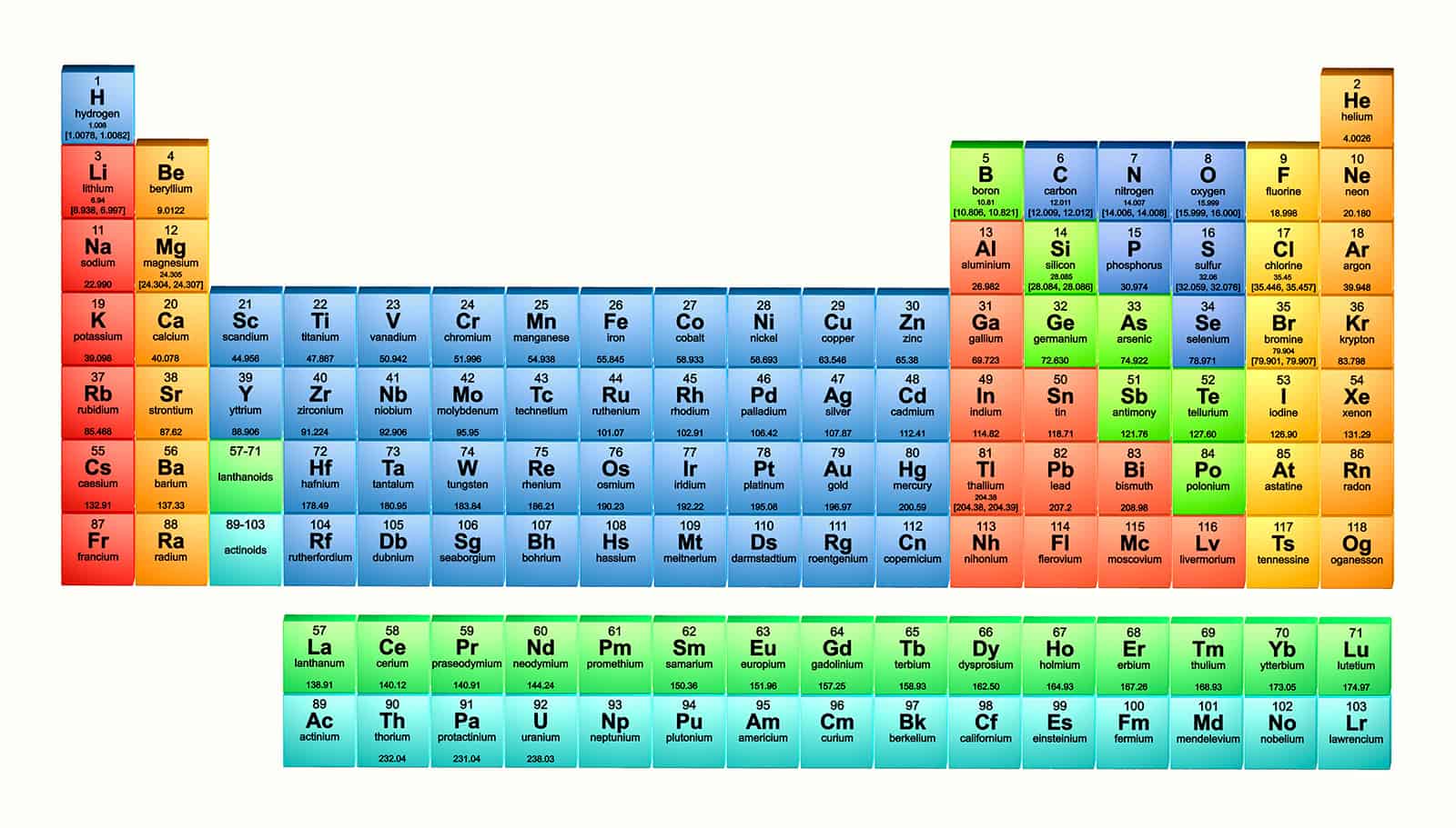
As I’m sure Pennant-Rea now appreciates, the periodic table is a thing of beauty and logic. It currently lists 118 elements, each of which is given a one- or two-letter symbol (can you name all 14 with just a single letter?). The elements are arranged into vertical “groups” and horizontal “periods”. The table can also be viewed as having three “blocks”, one of which – containing lanthanides and actinides – is often offset from the rest of the table.
Each element’s place in the table is its atomic number, but when Mendeleev drew up that first table at St Petersburg University, no-one realized what the number corresponded to. We know now, of course, that fluorine, say, is ninth in the table as its atoms each have nine protons. And its atomic weight is 19 as there are 10 neutrons. Intriguingly, fluorine is one of only 22 elements that have just a single stable isotope.
Many physicists can be snooty about chemistry, and will nod at Ernest Rutherford’s alleged dictum that all science is “either physics or stamp collecting”. But the periodic table is an attempt to bring order to chemistry and there is much to be learned from it in terms of atomic radii, ionization energies and shell structure. I’d even argue that the table these days is as much about physics as it is about chemistry. Indeed, when it comes to the super-heavy elements, whose fleeting existence can be proved only by combing through nuclear decay chains, it’s physicists who have led the way.
Early in 1869 the Russian chemical physicist Dmitri Mendeleev was growing increasingly frustrated while preparing the second volume of his textbook Principles of Chemistry. Though his first volume had been 600 pages long, Mendeleev had managed to cover barely eight of the 60 or so known elements in it. Facing a publisher’s deadline for the sequel before a looming trip to Europe, he decided to sketch out a table, putting the elements in columns and rows, ordering them by atomic weight in a way that showed their chemical similarities. He dated the table 17 February in the Julian calendar then used in Russia (corresponding to 1 March in the Gregorian calendar used throughout Europe).
Mendeleev was not completely satisfied with this table, and would go on to create about 60 more versions of the scheme. But his 17 February table became the basis for the one that now appears in the pages of every chemistry textbook and hangs in nearly every chemistry classroom around the world. But why did this table rise to fame, rather than the thousand or so other versions that one can find in the Internet Database of Periodic Tables? It includes many that look similar but also spiral, helical, circular and even 3D tables. The standard, textbook answer is that Mendeleev’s was the first table that graphically tried to display the chemical relations between all known elements ordered by atomic weight. But the real reason is more complicated.
One person with the answer is Ann Robinson, a science historian who works in the Widener Library at Harvard University in the US. Robinson is far from the first person to study the history of the table, but she is one of the most recent, having received her PhD on the subject last year from the University of Massachusetts in Amherst. Her thesis is timely: this month is the 150th anniversary of Mendeleev’s 17 February table, and July sees the centenary of the International Union of Pure and Applied Chemistry (IUPAC), which oversees global nomenclature and standards in chemistry.
Weighty matters
I recently visited Robinson at the Widener, which is the geographical and intellectual heart of the Harvard campus. Meeting me in the lobby of this imposing, colonnaded building, Robinson showed me one of the library’s treasures – a Gutenberg Bible, prominently displayed in an ornate chamber and one of just 49 surviving copies of this historically significant book.
By the 1860s, Robinson explained, chemists had settled on atomic weights as the most important characteristic for ordering the elements. Some chemists had even noticed that, when sequenced that way, groups of elements had similar properties. A few tried to express this insight systematically, including the British scientist John Newlands. Writing in a series of short articles published in Chemical News in the early 1860s, he proposed – and graphically illustrated – a “law of octaves”, whose principle was that every eighth element in his list exhibited similar chemical behaviour. But others ridiculed Newlands’ law, with many chemists thinking that he had pulled it out of thin air. It didn’t help either that Newlands had compared the relationships of elements to those of notes in a musical octave, a link that seemed whimsical to everyone but Newlands himself.
Over in Russia, meanwhile, and initially ignorant of Newlands’ work, Mendeleev was working at St Petersburg University, where he had been appointed a professor in 1864. He had become dissatisfied with existing chemistry textbooks, which divided elements into either metals or non-metals and classified them by their “valency”, or ability to combine with other elements. As the Princeton University science historian Michael Gordin recounts in his recently revised book A Well-Ordered Thing: Dmitri Mendeleev and the Shadow of the Periodic Table, Mendeleev set out to write his own textbook, sending Volume 1 to the publisher in January 1869.
Early period: Dmitri Mendeleev’s original hand-drawn table (left) was dated 17 February 1869 and is almost unrecognizable from the version we know and love today. The version on the right was published in his first scientific paper about the periodic table. To reach something resembling the modern table, you have to imagine rotating this diagram 90° clockwise and then flipping the elements left to right. (Courtesy: Sputnik/Science Photo Library; Universal History Archive / UIG / Science Photo Library)
But having covered only eight of the 63 known elements, Mendeleev began to condense his presentation in Volume II in the face of a contract deadline and page limitations, seeking to clarify the remaining elements in a way that would draw out their relationships. And so it was that on 17 February 1869 Mendeleev sent the Russian Chemical Society a single-page diagram, entitled “An attempt at a system of elements, based on their atomic weight and chemical affinity”. The scheme, Gordin notes, “arose out of the need for a pedagogical ‘classification’ [for] presenting material to beginning chemistry students”. Mendeleev then submitted a paper to the society and in 1869 published an abstract of it along with a version of the table in Zeitschrift für Chemie (12 405).
Robinson pulled out a copy of Mendeleev’s original diagram. Consisting of six columns of anywhere from two to 19 elements, it looked nothing like the modern periodic table we know and love. “You have to rotate it 90° clockwise, and imagine the elements flipped left to right, and the entire table unsquished,” she explained. When I did, it indeed looked roughly similar to our familiar table.
Fill the blanks
But Mendeleev was still dissatisfied with his new scheme. One troublesome feature, Robinson explained, was that in several instances, placing elements by their chemical behaviour collided with their placement by atomic weight. Tellurium (Te), for example, to which Mendeleev hesitantly assigned an atomic weight of “128?”, had to be placed before iodine (I), which had an atomic weight of 127. (We now know that the atomic weight is 127.6 for Te and 126.9 for I.)
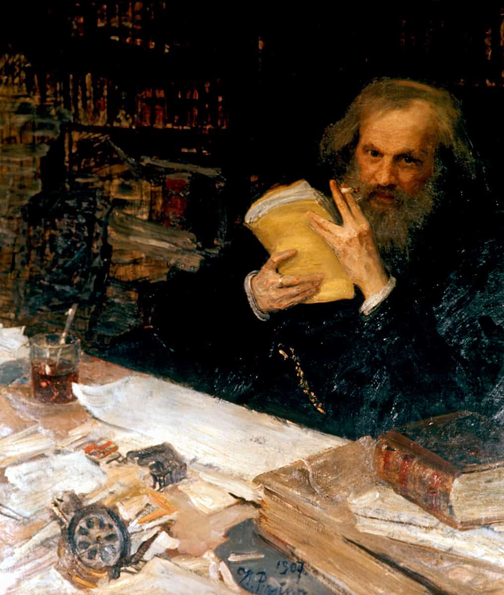
Ordered thinker: Dmitri Mendeleev (1832–1907) was a visionary in that his periodic table predicted four elements that were later discovered: gallium, scandium, germanium and technetium. (Courtesy: Sputnik/Science Photo Library)
Another puzzling feature, Robinson said, was that the table literally had holes into which Mendeleev had inserted question marks. In the table published with the abstract, these locations are for elements beneath boron (B), aluminium (Al), manganese (Mn) and silicon (Si) – the so-called rare earths, with approximate atomic weights of 45, 68, 70 and 180. Mendeleev decided that these holes weren’t the result of inadequacies in his classification scheme, but would be filled by hitherto undiscovered elements. Indeed, Mendeleev was so confident the new elements existed that he described their chemical behaviour and even gave them names by attaching the prefix “eka” (from the Sanskrit for “proto”) to those they most closely resembled. The element below aluminium, for example, became eka-aluminium.
A further curiosity of Mendeleev’s early tables, to us, is that one slot was occupied by an element labelled “Di” with an atomic weight of 95. As Robinson explained to me, that referred to didymium, which later turned out not to be an element but a combination of praseodymium (Pr) and neodymium (Nd). It’s a real substance, though, used in safety glasses to block out yellow light.
The first support for Mendeleev’s vision came in 1875 when the French chemist Paul Émile Lecoq de Boisbuadran discovered eka-aluminium, which he renamed gallia (in honour of the Latin name for the region of Gaul) – gallium (Ga) in modern English. The finding attracted attention to Mendeleev’s scheme, although most chemists were still unconvinced. As Robinson put it, the prediction was seen as “a lucky guess, a fluke”.
Then, four years later, the Swedish chemist Lars Fredrik Nilson discovered eka-boron – what we now call scandium (Sc). “Could he be lucky twice?” Robinson pointed out. “People thought, ‘maybe there’s something to this after all!’” More convincing was that Mendeleev had not simply predicted these elements, but also accurately forecast their properties and atomic weights. Further evidence in support of his table came in 1886 when eka-silicon (now germanium, Ge) was discovered, although the world had to wait until 1937 for the discovery of eka-manganese, which is now known as technetium (Tc) and one of whose isotopes is vital in medical physics.
Challenges ahead
Mendeleev’s table was thus the first time that a chemical classification scheme had been used to predict yet-unknown elements, and the Russian’s confidence in his basic scheme grew. Robinson pulled out a copy of the first English translation of his Principles of Chemistry, which was published in 1891 and based on the book’s fifth Russian edition, revised by Mendeleev. The table in that edition had lots of other un-named blank spaces, including the place where radium (Ra) would go 20 years later. “The chief theme of this work,” Mendeleev wrote in the preface, is the “philosophical principles” of chemistry. In it, he sought to “cast aside classical illusions”, and present the material “which not only gives mental satisfaction but is also practically useful”. He said his presentation was based on “the law of periodicity” of chemical elements and declared that his table placed them “in series, groups, and periods”. This version of the table resembled the one Robinson had shown me earlier, but with the elements flipped.
Mendeleev’s system was not entirely without problems, however. In 1870 he’d already had to gamble by doubling the atomic weight of uranium (U) from about 120 to 240 to make it fit (it’s actually about 238). Mendeleev also had trouble figuring out what to do with the lanthanides – a band of 15 elements including lanthanum (La), cerium (Ce) and neodymium (Nd) – and stuck them below the main part of the table. They were chemically similar to each other, but didn’t fit with the rest of the table. “They still don’t, and are still down there at the bottom,” Robinson wryly noted.
One troublesome feature for Mendeleev was that in several instances, placing elements by their chemical behaviour collided with their placement by atomic weight
Soon there were more disturbing events. One problem was J J Thomson’s discovery of the electron, the first subatomic particle, in 1897. Mendeleev did not think it existed. But some scientists tried (unsuccessfully) to incorporate it into the periodic table, giving it an atomic weight of zero. Another near-simultaneous event was Henri Becquerel’s discovery of radioactivity, which led to the conception of radioelements – radioactive substances that were thought to be elements. Chemists now had to postulate the existence of elements whose properties could not yet be determined, and possibly never could be. Mendeleev was also unconvinced by the idea of radioactivity, and in 1902 wrote an article proposing a “chemical conception” of the ether that would account for it. Even Marie Curie thought radioactive substances were impossible to characterize as chemical elements on account of “their destruction being too rapid”, and proposed the development of a “chemistry of the invisible”. Some periodic tables of the early 20th century did not include radioactive substances at all.
Radio-elements were puzzling for other reasons as well. They seemed to indicate the existence of substances with different chemical properties that looked like they occupied the same place on the periodic table, and substances with the same chemical behaviour that looked like they occupied two different places. “Elements aren’t supposed to do that,” Robinson said. “It was supposed to be one element per square!” But if radioactive elements challenged early visions of the periodic table, it also facilitated the discovery of new elements of this kind.
By 1914 things had pretty much been cleared up. Ernest Rutherford had discovered the atomic nucleus three years before, and – thanks to the notion of quantum physics – Niels Bohr had made Rutherford’s scheme workable. Frederick Soddy then demonstrated the existence of isotopes: atoms of one particular element with the same number of protons but different numbers of neutrons. The notion solved the placement problem, because all isotopes of an element can be put in the same square of the periodic table, with the atomic weight of an element – what’s now also called the relative atomic mass – being the average mass of all atoms of the element, taking into account their different abundances. Henry Moseley’s X-ray studies showed that the “atomic number” of an element is not an arbitrary number but associated with a specific measurable property of the atomic nucleus. It is the number of protons in an atom and thus its numerical place on the periodic table when elements are arranged by atomic weights
Moseley’s work cemented the justification for Mendeleev’s scheme, and among other things definitively established the legitimacy of placing tellurium (52 protons) before iodine (53 protons) on the periodic table. Yet the increasing primacy of atomic number over atomic weight, Robinson said, was accompanied by a fear among chemists that physics was encroaching on their role in characterizing elements.
The road to fame
In her PhD dissertation, Robinson traces what followed. After 1869 many chemists produced versions of Mendeleev’s table, and teachers found such tables useful. The first textbooks to include a periodic table were published in the 1870s, but the first version of the table that we are most familiar with did not appear until 1923 when the US chemist Horace G Deming published a textbook called General Chemistry: an Elementary Survey Emphasizing Industrial Applications of Fundamental Principles.
Robinson showed me a second edition of Deming’s book, which wasn’t aimed at academic researchers. “It was geared towards students who wouldn’t necessarily go much further in chemistry, or who would go into industry,” she explained. The textbook proved a huge hit and went through six editions – the last in 1952 – popularizing Deming’s revised version of Mendeleev’s table. Chemical companies also began using it in their material and, by 1928 the American pharmaceutical giant Merck had shrunk the table and distributed it in letter size and index-card size. In 1934 it was the first periodic table to be incorporated into the CRC Handbook of Chemistry and Physics – a standard reference manual. “Those events made it the table,” Robinson said. “It was a pragmatic system that was extremely useful in chemical education.” The key point of her dissertation, in fact, is that “pedagogy played a more important role than research did in the development of the form of the periodic table”.
Modern vision: Today’s periodic table (as of May 2017) includes 118 known elements, with the most recent additions being nihonium (element 113), moscovium (115), tennessin (117) and oganesson (118). This version is colour-coded to show elements with similar properties. Those elements with no atomic weight listed are unstable. (Courtesy: Alfred Pasieka/Science Photo Library)
The table has even proven resilient enough to survive the discovery, over the last 25 years, of elements whose atomic number is over 110, filling out the remaining space in the table’s seventh row. “One of the great features of the periodic table,” Robinson reminded me, “is its elasticity, its ability to accommodate elements that Mendeleev would never have expected, such as synthetic elements.”
But the periodic table, whether Mendeleev’s or the others, did not solve one problem. What, finally, is an element? It is one example of a scientific issue that cannot be resolved by more research, but requires reflection on basic principles that guide theory and experiment. Answering the question falls within the bounds of philosophy of science. Indeed, some philosophers have wondered whether the “superheavy” elements at the end of the periodic table (those with atomic weights of 104 and over) can really be called elements. Given that they are not found in nature, can only be made in labs and disintegrate almost immediately, they raise serious questions about whether they even “exist”.
Another philosophical issue that the periodic table raises is the boundary between physics and chemistry. Is an element a species of something whose fundamental bits share the same structure, which is how physicists think of them? Or is an element something with properties like colour and smell that can be experimented on – the chemists’ view? Physicists generally picture elements as invisible things that can’t be seen and remain the same when combined, while chemists think about their elements as real substances you can hold in your hand, like a lump of tungsten. Both the physicists’ and the chemists’ views seem integral to the idea of an element, though they involve different pictures. Mendeleev had already encountered this problem, and those who followed often tried to solve it with such distinctions as pure and simple substances, or chemical element and elementary substance. Such distinctions represent the practical divide between chemistry and physics.
The issue persists today, with even IUPAC refusing to take a stand on the definitive periodic table. Its Compendium of Chemical Technology – colloquially called the Gold Book because that’s the cover’s colour – gives not one definition of an element but two. The first defines an element as “all atoms with the same number of protons in the atomic nucleus”, while the second defines it as “a pure chemical substance composed of atoms with the same number of protons in the atomic nucleus”. But 150 years after Mendeleev’s first periodic table, the fact that this distinction still persists is, for Robinson, a reaction to the intrusion of physics into chemistry. “You physicists can play with our elements all you want,” she warned. “But there’s still a chemical element in there that you cannot take away!”