Pop physics: can you explain fermion identity better than using twins occupying the same space? (Courtesy: iStockphoto/Christophe Delvallé)
Of all features of the quantum realm, the forms that particles take are surely among the most bizarre. There are only two possibilities: identical objects that can mash together (bosons), and identical objects that cannot (fermions). Bosons obey a mathematics called Bose–Einstein statistics, while fermions follow Fermi–Dirac statistics. These two possibilities were found independently in 1924–1925 with Satyendra Nath Bose and Albert Einstein discovering the properties of bosons, and Wolfgang Pauli’s exclusion principle articulating the basic behaviour of fermions.
In 1926 Paul Dirac synthesized these possibilities in a mathematical framework. Crudely, if you exchange two identical objects and the “phase factor” of the wave function is the same, or “symmetric”, the objects can occupy the same quantum state and physical position and are bosons. (A group of bosons falling into the lowest possible energy state creates a Bose–Einstein condensate.) If the phase factor is negative, or “antisymmetric”, the objects cannot occupy the same position and are fermions.
The mathematics of the quantum world restricts objects to these two possibilities, which means that bosons and fermions play vastly different roles in the quantum realm. Bosons serve as force-carrying particles – photons, for example, are particles corresponding to electromagnetic forces. As for fermions, Pauli’s exclusion principle and the uncertainty principle regulate the atom’s energy levels, which determine the chemical properties of elements and the structure of matter.
Bosons and fermions are familiar to physicists. But writing in the journal Philosophy of Science in 1944 – the year before Pauli won the Nobel prize – the physicist and philosopher of science Henry Margenau said it was “strange” that there was “so little discussion of the exclusion principle in the philosophical literature”. He could have added that there was scant presence of it – or of Bose–Einstein condensation – in popular culture either.
Popular culture often exploits quantum weirdness, finding such terms as quantum leap, complementarity, superposition and parallel worlds packed with creative force. US President Barack Obama has even invoked Heisenberg’s uncertainty principle to explain his occasional reluctance to confront advisers directly about their opinions, while his recent opponent – former governor Mitt Romney – was satirically labelled a “quantum politician” for the way he articulated randomly fluctuating views, held superposed positions and asserted complementary statements on subjects depending on the context.
Yet the Pauli principle and Bose–Einstein condensation are all but absent from popular culture. Identity is the quantum shoe that hasn’t dropped.
But why not?
Tag-ability
Classical mechanics depends on the distinguishability of even primal bits of matter. In other words, you could, if you wanted, put tags on things and follow them around. Sure, atoms and molecules of the same type were thought to be identical, but each one was in principle “tag-able”. Those scientists, such as James Clerk Maxwell, who stopped to ponder the marvel of a universe full of identical yet distinguishable objects, had no explanation. Some cosmic factory had produced perfect duplicates of atoms, and all Maxwell could figure was that God was somehow responsible.
But one hint that something might be amiss came with a puzzle uncovered in the late 19th century by the American scientist Josiah Willard Gibbs. He imagined two adjacent boxes containing equal amounts of a gas at the same temperature. What happens, he asked, if a partition between the two boxes were removed? The molecules mix, of course. Indeed, if you label each molecule by a different number – even numbers, say, for molecules from the first box and odd numbers for molecules from the second – the evens and odds start together and eventually mix uniformly.
As an irreversible process, this should – according to classical physics – increase entropy. But because the entropy actually stays the same, the molecules must therefore be indistinguishable. In other words, they are different from all macroscopic objects. But until the appearance of the quantum – which early on was recognized to imply indistinguishability – nobody knew what to make of this puzzle.
The critical point
Both versions of quantum identity are bizarre. On the macroscopic level, fermion identity is like fraternal but non-identical twins being able to co-inhabit a space. Boson identity is like that old vaudeville gag of a crowd of people emerging from a small space like a phone booth – except that an infinite number of people could do so.
Given our cultural obsession with cloning and identity, why has popular culture, which celebrates the bizarre, not noticed quantum identity? Why isn’t it on T-shirts or coffee mugs, or mentioned in TV shows that appeal to geeks?
It is true that the exclusion principle seems almost commonsensical – a quantum extension of the classical reality that no two things can be in the same place at the same time; it may seem, that is, simply like saying that you cannot do on the microscopic scale what you cannot do on the macroscopic scale. Yet this misses the weirdness that what cannot be in the same place at the same time is something identical.
There must be more to it. Non-scientists often apply scientific language to experiences for which ordinary words are inadequate. So does the absence of quantum identity in popular culture signify our satisfaction with our present language of identity? Or have our imaginations shrivelled? More positively, what kinds of experiences do we humans have that might cry out for metaphors involving quantum identity?
Here, then, is a challenge for readers. Can you devise a situation drawn from the everyday world in which the phrases “quantum identity”, “Pauli exclusion”, Bose–Einstein behaviour”, or some variant of those phrases, would be poetic, enlightening or simply meaningful? I will write about responses in a future column.
The tablet revolution began on 27 January 2010, when Apple’s then chief executive, Steve Jobs, stood in a packed lecture hall in San Francisco and unveiled “a third category of device”. With the arrival of the iPad tablet, technology finally caught up with science fiction – keyboards, mice, printers and disk drives had all been replaced with a simplified touchscreen interface and a wireless network connection. Apple’s device quickly gained competitors, as tablets’ portability and ease of use made them an instant favourite among people who use their computers mainly for e-mailing, browsing the web, watching films and playing games. It took a little longer to adapt more serious desktop tools such as word processors and spreadsheets for use with a simplified touchscreen interface, but before long, almost all common desktop applications had tablet siblings.
There was, however, one major exception: LaTeX. Despite impassioned pleas from the academic world, the typesetting program used by tens of thousands of mathematicians, physicists and other scientists seemed to have been left out of this technological revolution. That began to change in September 2012, when two native LaTeX “apps” finally made it to the iPad – one of which, Texpad, was the result of a year-long development project for me and my business partner, Jawad Deo. However, the new apps still lack many of the packages and tools that users have come to expect from LaTeX, so although LaTeX has now joined the tablet revolution, it continues to lag behind. Why?
Stuck in the sandbox
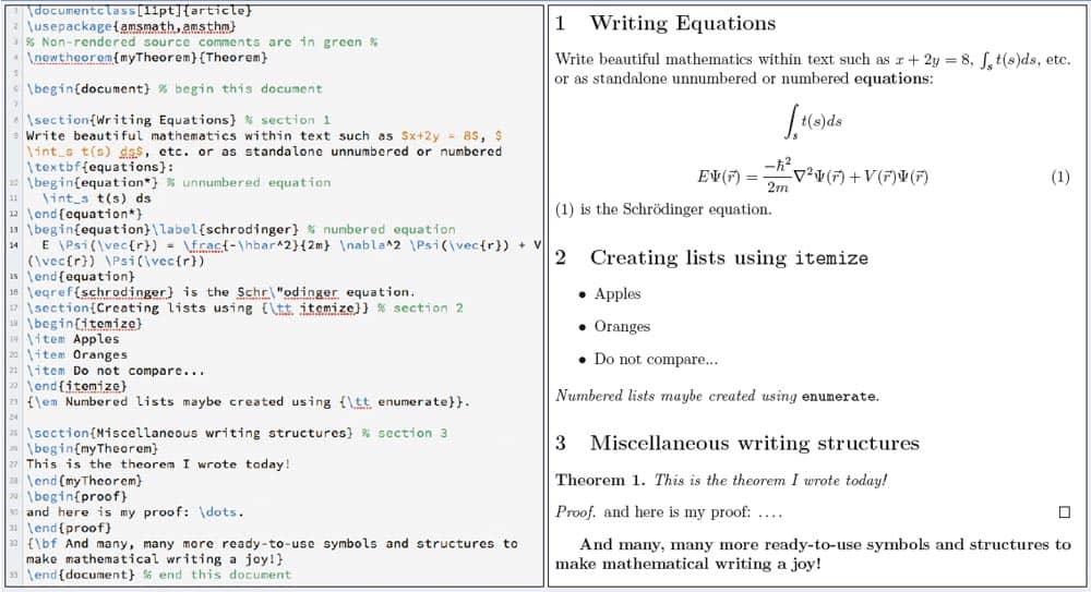
LaTeX is an offshoot of a typesetting program called TeX, which was introduced by the computer scientist Donald E Knuth in 1978. In Knuth’s words, it was “intended for the creation of beautiful books – and especially books that contain a lot of mathematics”. LaTeX was born when a set of extension packages for TeX was released in the early 1980s. TeX and LaTeX differ from word processors such as Microsoft Word in that they replace cumbersome equation editors and layout options with a simple “typesetting language” (figure 1). For example, to make boldface text in LaTeX, you just place the text within the brackets of a “textbf{ }” command. Many common mathematical symbols are particularly easy to create: inserting an integration sign requires the command “int”, and the command for a subscript “s” is simply “_s”. Newcomers to LaTeX face a steep learning curve, but once they have become accustomed to the program’s high-quality typography, they rarely switch back.
1 Beautiful mathematics This block of LaTeX “code” (left) and the corresponding typeset document (right) shows how LaTeX produces several features of mathematical textbooks, including equations, lists and numbered sections. Although it takes a while for beginners to grasp the program’s structure and master its commands, LaTeX is more flexible than the “what you see is what you get” equation editors used in word processing programs, and most users feel that the results are worth the effort.
In the years since its creation, TeX migrated painlessly from mainframe to desktop to laptop, so it is not obvious why it is taking so long to progress to tablets. Nothing about the TeX typesetting language is incompatible with a touchscreen interface. Instead, the obstacles lie below the tablets’ sleek metal-and-glass exteriors, in the operating systems powering the tablet revolution.
A traditional desktop operating system has a single file system that is visible to the user and accessible by all installed software. This architecture makes it possible for a malicious or malfunctioning program to “run loose” and attack other files, but it also allows a single task to be distributed across multiple applications and tools. LaTeX typesetting is a great example of this distributive process. For example, to produce the first draft of this article, I typed it in the desktop version of our Texpad LaTeX editor, which passed the data first to LaTeX, then to a program called dvips that converts files from one format (DVI) to another (PostScript), then to the ps2pdf PostScript to PDF converter, and finally back to Texpad for display (figure 2).
2 Step by step Producing a LaTeX document is a multi-step process that requires an editor (such as Texpad) to share information first with the typesetter, LaTeX, then with conversion programs such as dvips and ps2pdf.
Tablet operating systems such as those found on the iPad and Android-based tablets, however, force all software to be self-contained: every application is restricted to a subset of the file system and hardware. This subset is called a “sandbox” and it acts like a virtual cage within which an application’s files are both contained and protected from other applications. Just as cages ensure that zoos don’t consist of a large pile of animal carcasses and one well-fed lion, sandboxes create a safe environment for the user where any single malicious or malfunctioning application is limited to damaging its own files.
This is great for security, but it inhibits software such as LaTeX, which relies on a co-operative style of software architecture. If a tablet LaTeX editor needs to communicate with a tablet LaTeX typesetter, then it must include that typesetter within its sandbox, along with all the tools and packages the typesetter requires. iOS, the iPad’s operating system and as such the most widely used tablet operating system, goes even further and requires all software to be packaged as a single program. In almost every case this makes sense, but it is a headache when you consider the four different programs in the simple typesetting example described above.
Consequently, for the iOS version of Texpad we combined the editor, LaTeX, a bibliography program called BibTeX and a basic set of LaTeX packages, all in a single program. Contrast this with a desktop installation where these components would be all be distributed, updated and operated as separate entities.
A complex ecosystem
The problem with packaging LaTeX in this monolithic manner is that after nearly 35 years, the TeX ecosystem consists of a mind-boggling number of packages, and almost every day we get an e-mail from a user asking us to add some esoteric package or tool. The youngtab package is a perfect example: it allows you to draw collections of boxes or cells called Young tableaux in your LaTeX document, and although it is indispensable for some mathematicians and theoretical physicists, it is useless for the majority of users. For now, we are happy to keep expanding what we offer, but we rarely get the same request twice, and if we added every package our customers want, our app would outgrow a tablet’s limited storage space. For example, the current edition of the most widely used distribution of LaTeX, TeX Live 2012, consumes 4 GB of space on my hard disk. Although tolerable on a laptop, that equates to almost a third of my iPad’s usable space – an unacceptable size for an application. The bloated nature of LaTeX also slows down the typesetting process. While a web browser can lay out a large document almost instantaneously, typesetting even the simplest document on my laptop takes 2 s, and my PhD thesis took well over a minute. This isn’t a problem on a fast desktop computer, but on a low-power, battery-conscious tablet, it can be.
The biggest problem for developers of a tablet-friendly LaTeX is not the number of LaTeX tools and packages, or even the sandboxed tablet operating systems, but the fractured nature of TeX itself. To illustrate this, suppose an experimental physicist is writing a paper, and she wants to include both a diagram and a photograph of her experiment. How should she do this? One common choice of package for drawing diagrams in LaTeX is PSTricks. However, PSTricks only works with the LaTeX/dvips/ps2pdf chain of typesetting tools described above, and her photo is in JPEG format, which will not typeset with that chain. JPEGs will typeset with a different version of LaTeX, known as pdfLaTeX – but PSTricks, of course, won’t.
To get around this apparent impasse, our experimental physicist could re-draw her experiment using a different package that is compatible with pdfLaTeX, or she could use a package to convert her photo to a format acceptable to the original typesetting chain. I don’t want to bore you with all her other options, but on the version of LaTeX currently running on my laptop, I count a choice of six typesetting chains, two diagram packages, and innumerable tools to knit all these choices and their incompatible file formats together.
The tangled web
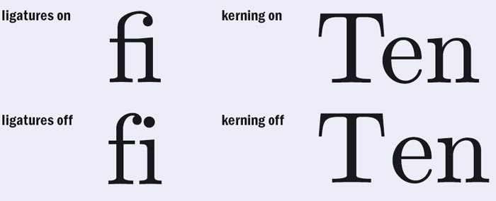
Why, you may ask, is TeX structured in such a tortuous fashion? After all, it was written by Knuth, a man who is held in the same esteem among computer scientists as Richard Feynman is among physicists. When Knuth began TeX in the 1970s he started from scratch. There was no font system suitable for TeX, and no suitable file format for the final typeset product either. Knuth’s solution was to create a new font system, Metafont, and his friend David Fuchs created a new document format, DVI. All of this was written in WEB, a programming system Knuth also created. The resulting system was so far ahead of its time that it took 20 years for a general-use font format (OpenType) to emerge with support for all the typographical tricks supported by TeX and Metafont, such as kerning and ligatures (figure 3), and to bring these techniques into wide usage.
3 Spot the difference Certain combinations of letters, such as those shown above, are easier to read when parts of them are merged (ligatures) or the spaces between them are adjusted to account for their shapes (kerning).
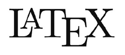
Few people have the creativity, programming ability and endurance required to construct a system as capable as TeX from nothing, and Knuth deserves the renown it has brought him. He certainly has my gratitude. Nevertheless, over time, Knuth’s groundbreaking technologies aged and disappeared. DVI gave way to PostScript in the 1980s and PDF in the 1990s; Metafont did not survive the arrival of PostScript either; and as for the WEB programming system – well, as far as I know, Metafont, TeX and the occasional TeX-related tool, such as the bibliography-generating BibTeX, are the only pieces of software written in it. Even the LaTeX logo (below right) has aged. Initially, it was a demonstration of TeX’s powerful support for superscripts, subscripts and kerning. Now, it is just a hassle to have to type the extra capital letters every time.
Ups and downs The LaTeX logo in its official format, complete with kerning, ligatures and multi-level type.
In the face of all these changes, Knuth decided to preserve TeX’s core in its original state, and he only consented to alterations that fix bugs in this core code. So although DVI, Metafont and WEB usage have declined, TeX continues to produce files in the defunct DVI format – forcing developers to write external utilities to convert the DVI file to a PDF. Users also came to expect colour and images in their documents, but once again TeX was not modified; instead, extra features were embedded in the ancient DVI format as “special strings” for a different tool to interpret and render further down the pipeline.
Inevitably, a PDF-producing variant of TeX, called pdfTeX, was written. But thanks to Knuth’s prohibition against altering TeX, pdfTeX soon became a separate and competing typesetting tool. Many packages will run on both systems, but some run on pdfTeX only, and others on the original TeX only. Unfortunately, this “forking” set a pattern in TeX development, splitting not only the code but also the efforts of its community of developers. Today there are five widely used typesetting engines – TeX, pdfTeX, XeTeX, luaTeX and pTeX – as well as some less common ones, such as kerTeX.
Out of many, one?
At this point, non-LaTeX users may be wondering why anyone bothers with such a complex and clunky system. LaTeX’s longevity rests on one simple fact: it produces beautiful documents. For most users, that is all that matters. Not everyone needs to know about what is going on “under the hood”, and for those physicists who do take a peek, the intricate nature of LaTeX can be appealing. Its interlinking architecture conjures up images of a patchwork of tools running in harmony – the typesetting equivalent of Charles Babbage’s difference engine.
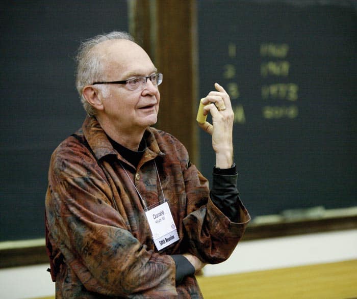
Man of principle? Donald E Knuth, original creator of LaTeX, lecturing at Case Western University in Ohio in 2010. (Courtesy: Dasha Slobozhanina)
However, a difference engine won’t fit in your pocket, and those of us working behind the scenes also recognize that this particular engine would spin more smoothly if it had fewer cogs. The incompatibility between LaTeX’s heritage and structure and the sandboxing on most tablet devices has merely heightened an existing problem. For us, the only solution has been to do what the LaTeX community should have done long ago: choose.
To create our LaTeX tablet app, we have selected a single typesetting engine, kerTeX, and a single file format, PDF. We have merged this with the BibTeX bibliography tool into a single software component, or “library”, that is plugged into Texpad, our editor. The result is a pleasantly snappy typesetter, and a starting point from which we are modernizing LaTeX’s internal architecture to make it both compatible with tablets and amenable to further development.
It is often said that “the path to hell is paved with good intentions” and today’s fractured LaTeX lies at the end of a long trail of well-intentioned rewrites. We are mindful that an ecosystem blighted by incompatible standards cannot be cured with another incompatible standard – even if it does come in tablet-friendly form. To avoid this trap, we are following XeTeX’s example of supporting standards rather than creating them. XeTeX (and the related XeLaTeX) have discarded the TeX-specific character encodings in favour of Unicode, an encoding system containing virtually all characters ever written – from the familiar Latin alphabet to ancient Egyptian hieroglyphics. Unicode has long since been the standard encoding in all other areas of the computer world, so having supported Unicode, XeTeX is also capable of working with modern font standards, such as the OpenType format mentioned above, rather than just the antiquated, and TeX-specific, Metafont files.
Other approaches are possible, especially on tablets based on the more loosely sandboxed Android operating system, on which a single application can consist of multiple interacting programs. As this article was being prepared for publication at the end of 2012, an Android developer, Vu An Hoa, released the TeXPortal application in which he packaged the entirety of TeXLive in its original multiple-program form within a single application sandbox. There is a great deal of effort being spent on adapting LaTeX for tablet computers, and this effort is incontrovertible proof of the importance and superiority of Knuth’s system.
As important as it is for TeX to keep abreast of changes in the computer world, the typographical quality of documents produced by the 1978 version of TeX still stands up against today’s word processors. That is why LaTeX has survived several technology revolutions already, and it is why it will also survive the advent of tablet computers.
The rate at which protons capture muons has been accurately measured for the first time by the MuCap collaboration at the Paul Scherrer Institute (PSI) in Switzerland. This process, which can be thought of as beta decay in reverse, results in the formation of a neutron and a neutrino. The team has also determined a dimensionless factor that influences the rate of muon capture, which was found to be in excellent agreement with theoretical predictions that are based on very complex calculations.
Muons are cousins of the electron that are around 200 times heavier. Beta decays demonstrate the weak nuclear force in which a neutron gets converted into a proton by emitting an electron and a neutrino. Now, replace the electron with the heavier muon and run the process backwards: a proton captures a muon and transforms into a neutron while emitting a neutrino. This process – known as ordinary muon capture (OMC) – is crucial to understanding the weak interaction involving protons.
The proton and the weak force
The proton’s interaction with the weak force is explained by the chiral perturbation theory (ChPT) – an approximation of quantum chromodynamics (QCD) applicable at low particle energies. At such energies, the weak interaction inside a proton is affected by the presence of the strong force. The strength of this weak interaction is determined by certain coupling constants, which must be experimentally established.
“Essentially, these constants represent the basic properties of the proton, and describe the fact that it is not point-like but has a complex internal structure,” says Peter Kammel from the University of Washington, Seattle, one of the physicists involved in this research. Three of these dimensionless parameters have been previously measured, but attempts at measuring the fourth, known as “pseudoscalar coupling”, provided conflicting results, until now. “Of course,” continues Kammel, “the pseudoscalar coupling constant could be calculated quite precisely by using chiral perturbation theory, which predicts a value of 8.26 ± 0.23.” In order to measure its value, the physicists had to first determine with a high accuracy the rates at which muon capture takes place.
Capture versus decay
The muons used in the study were produced by smashing protons into carbon targets at an energy of 590 MeV. These collisions produce both positive and negative pi-mesons (or pions), which promptly decay into positive and negative muons, respectively. Muons with an energy of 5.5 MeV are then fired into a MuCap time projection chamber (TPC), which contains ultrapure hydrogen gas at 10 bar.
The negative muons supplant the electrons that orbit the hydrogen nuclei to form a proton–muon bound state, while the positive muons remain free. A small fraction of the bound muons – around 0.16% – will get captured by the proton and disappear, as they form a neutron and a neutrino. All of the remaining muons, both positive and negative, will decay after about two millionths of a second into electrons and neutrinos. The decay times were calculated precisely by measuring the time between the muons entering the TPC and the electrons from the decay exiting the chamber. These decay times were then compared to the well-known free muon decay rate and the difference between the two determines the elusive muon-proton capture rate.
A total of around 12 billion decay events involving negative muons were detected, corresponding to 30 TB of raw data that were analysed. The analysis was performed blind to prevent any unintentional bias from distorting the results and, following the unblinding, the measured muon-capture rate was found to be 714.9 ± 5.4 (stat) ± 5.1 (syst) s–1.
Confirming predictions
Using this figure, the team could calculate the value of the pseudoscalar coupling constant, which worked out to be 8.06 ± 0.48 ± 0.28, consistent with the predictions of ChPT. Although experimental methods to determine the pseudoscalar coupling constant started in the 1960s, it was not until the MuCap experiment that the objective was achieved.
“The nucleon weak-interaction coupling constants played a significant role in understanding the weak and strong interactions,” continues Kammel. “The modern description of the process we have investigated is based on ideas proposed by Yoichiro Nambu, for which he won the Nobel Prize for Physics in 2008.” The approximate methods of calculation presented by ChPT agree very well with the experimental result, confirming yet another prediction of the Standard Model of particle physics.
With fully fledged quantum computers still potentially decades off, several groups of physicists around the world have found an alternative way of exploiting the processing power of quantum mechanics. They have built a relatively simple photonic device to carry out one specific calculation that is very difficult to perform using classical computers and which, they say, might demonstrate the greater inherent speed of quantum-based devices within the next 10 years.
Quantum computers process quantum bits – or qubits – which can exist in two states at the same time. This could, in principle, lead to an exponential increase in the processing speed of a quantum computer compared with classical devices. This quantum processing could be used, among other things, to rapidly factorize large numbers into their constituent primes and so break codes that are, in practice, uncrackable using conventional computers. However, many technical challenges remain for those trying to develop quantum computers and today the best that a quantum computer can do is to factor small numbers such as 15 and 21.
Some physicists believe that an intermediate quantum computer called a “boson sampling” machine could offer a shortcut to achieving the greater speed of quantum computing. This does not involve what is known as a universal quantum computer, but instead carries out one fixed task. The device consists of a network of beam splitters that converts one set of photons arriving at a number of parallel input ports into a second set leaving via a number of parallel outputs. Its task is to work out the probability that a certain input configuration will lead to a certain output.
Bosonic properties
In 2011 Scott Aaronson and Alex Arkhipov of the Massachusetts Institute of Technology showed that calculating that probability becomes exponentially more difficult using a classical computer as the number of input photons and the number of input and output ports increases. That difficulty is due to the unusual behaviour of photons, which belong to a class of fundamental particles known as bosons, any number of which can occupy a given quantum state. When two photons reach a beam splitter at exactly the same time, they will always follow the same path afterwards – both going either left or right – and it is that behaviour that is so hard to model classically. The MIT researchers found that predicting the machine’s output in fact requires the calculation of a series of “permanents” – single numbers associated with specific matrices that are similar to determinants but which are much harder to work out.
“Having to work out these permanents means that even the best desktop computers would struggle to get above about 30 photons,” says Ian Walmsley of the University of Oxford in the UK. “But a boson sampling machine instead is a kind of analogue computer that uses the physical properties of bosons themselves to work out the answer.”
Four independent groups of researchers have now backed up Aaronson’s theoretical work with experimental results. One is led by Walmsley and includes researchers from Oxford and Southampton universities. Another is an Australian/US group led by Andrew White of the University of Queensland that includes Aaronson. Both of these groups have had their results published in Science, while the other two groups – based in Austria/Germany and Italy/Brazil – have released their results on the arXiv preprint server. All groups used similar experimental set-ups based on either custom compact optical chips or commercial photonics with five or six inputs and outputs.
Injecting photons
The tests involved injecting up to three photons, or four in the case of the Oxford group, into specific individual inputs and then registering at which outputs photons emerged. Repeating this process over and over again, the researchers were able to work out what fraction of the time specific output configurations appeared, and therefore the probability that those configurations would occur.
Comparing these results with the probabilities calculated using matrix permanents, the groups found experiment and theory to be in very good agreement, once the theory had been corrected to account for experimental errors arising from photons that sometimes were not indistinguishable (which they must be) and which sometimes entered the system as pairs rather than individually. The finite time over which data were collected also limited the accuracy of the results.
“The bottom line is that we have built boson sampling machines, that they work and that the errors are not fatal,” says Walmsley.
Direction is clear
Being able to account for these errors suggests that the devices can be scaled up to the point where they overtake classical computers, according to Walmsley. The aim, he explains, is to improve the technology in order to process around 30 photons, which is generally considered to be about the limit for a present-day desktop classical computer, and then up towards 100, which would put the boson samplers in a league of their own. “To do that you need to make sure that the photons are all exactly the same, that they arrive at the beam splitters at exactly the same time, and that the detector efficiency allows you to sample enough data,” he says. “There are challenges in overcoming all of these things and that will mean a lot of work, but I think the direction we need to take is clear.”
White agrees. “I think that within a decade we can get there,” he says.
In fact, Walmsley believes that boson sampling machines “might not simply be a test exercise” for universal quantum computers and that they may, in fact, be used to compute additional, useful algorithms – although he points out that no such algorithms have been discovered yet.
However, Raymond Laflamme of the University of Waterloo in Canada is a little more cautious. He says that he read about the latest results “with enthusiasm” and believes that boson sampling “is teaching us something important about quantum information processing – that we might not need a fully operational quantum computer to have an interesting speed up from quantum mechanics”. But he is not sure the current devices really can be scaled up. “It is not clear to me that the experimental results will not be swamped by the imperfections when trying to reach 20 or 30 photons,” he says. “But on the other hand I can’t prove it, and that is the challenge for the experimentalists.”
The thermal Josephson effect, which occurs when heat is transported across a gap between two superconductors, has been measured in the lab for the first time. The experiment was done by two physicists in Italy and confirms a theoretical prediction made in 1965. As well as confirming the bizarre prediction that some heat flows from the cold side of the junction to the hot side, the breakthrough could further the development of thermal circuits that use heat in much the same way as charge is used in electronic devices.
The conventional Josephson effect was predicted in 1962 by the British physicist Brian Josephson and was observed in the lab less than a year later. The effect occurs in a Josephson junction, which is created when two superconductors are separated by a thin layer of non-superconducting material or free space. Josephson showed that Cooper pairs – paired electrons that experience no electrical resistance within superconductors – can tunnel across the junction. All of the Cooper pairs are in the same quantum state and are thus represented by the same wavefunction. The tunnelling current is a sinusoidal function of the phase difference of the wavefunction from one side of the gap to the other. As a result, a current of Cooper pairs will flow across the gap even if there is no applied voltage.
If a voltage is applied across the junction, then things get more complicated and three different processes affect how current flows across the junction. The first, predominant term is the Josephson supercurrent, which would be present even without the voltage. The second contribution is from Cooper pairs that break apart into their constituent normal electrons, which can then tunnel through the potential barrier under the influence of the applied voltage. Last, there is an “interference current” that arises from the interaction between the first two processes.
Thermal bias
In 1965 Kazumi Maki and Allan Griffin of the University of California, San Diego calculated what would happen if a Josephson junction were given a thermal bias – that is, one side being slightly hotter than the other – rather than the usual voltage bias.
Ordinary metals can transport heat by energetic electrons moving from hot areas to colder regions – where they heat the surroundings by scattering from atoms and creating lattice vibrations. This does not apply to superconductors, however, because Cooper pairs move without scattering. In a thermally biased Josephson junction, therefore, the supercurrent does not contribute to heat flow. However, both electron tunnelling and the interference current can be involved in heat transfer across a junction.
Heat flow from electron tunnelling is a straightforward process that will always move heat from the hotter to the colder side of the junction. The curious part of Maki and Griffin’s prediction, however, is that the interference current can sometimes carry heat from the cold to the hot side. This is because, like the supercurrent, it depends on the superconductor wavefunction.
Tough to test
Testing this prediction has proved difficult, according to Francesco Giazotto and María José Martínez-Pérez of the NEST Institute of Nanoscience and Scuola Normale Superiore in Pisa – who are the first to do so. This is because, unlike electric currents, heat currents cannot be measured directly. “There is no analogue of an ammeter for a heat current so you are measuring an observable that is related only to the heat current like temperature,” explains Giazotto. He also says that it is much more difficult to keep track of heat flow than of charge.
Giazotto and Martínez-Pérez made their measurements on a superconducting quantum interference device (SQUID) – a loop of superconductor broken by two Josephson junctions. One half of the loop is kept at a slightly warmer temperature, causing normal electrons to carry heat across the two junctions to the cooler side as predicted.
The experiment involves altering the amount of magnetic flux that passes through the SQUID, which in turn affects the nature of the wavefuntion at a Josephson junction. By showing that the heat flow modulates between maximum and minimum values as the magnetic flux is changed, Giazotto and Martínez-Pérez have confirmed that the interference current can actually transfer heat from cold to hot. However, the overall heat flow does not reverse because the flow is dominated by normal electrons tunnelling through the junctions.
“Very clean result”
Raymond Simmonds of the National Institute for Standards and Technology in Boulder, Colorado, is impressed by the experimental challenges the researchers have overcome. “It’s really surprising that they got to measure a very clean result,” he says. “They had to do some pretty good engineering to make their heaters and their thermometry well characterized, all on a very small device, and to engineer all their contacts to ensure the system isn’t shorted out by the substrate.”
Giazotto and his colleagues are now look at possible practical applications of the result could be. He speculates about the possibility of “a sort of coherent caloritronic circuitry – the analogy of electronics but with heat”. He suggests it might be possible, for example, to produce heat transistors or heat rectifiers or even to produce devices without an electronic analogue.
“What is temperature?” is the sort of question that a seven year old would ask – and a physicist would struggle to answer in a simple way. That’s why a paper published today in Science about “negative temperature” seems very puzzling at first glance.
One way of looking at temperature is as a way of describing how energy is distributed among a collection of particles. Most particles will have a small amount of energy and the probability that a particle has a higher energy will drop exponentially with energy – the familiar Maxwell–Boltzmann distribution of an ideal gas. Temperature times Boltzmann’s constant is the parameter that fits the distribution to experimental data. Implicit to this distribution is that there is a minimum energy (zero) and no maximum energy.
Now, a team of physicists has used ultracold atoms to create what is essentially a mirror reflection of this familiar scene – a system with a maximum energy and no minimum energy. Furthermore, the probability that a particle in this system has an energy approaching this maximum is very high and drops off exponentially as the energy decreases.
So if you interpret this in terms of the Maxwell–Boltzmann distribution, you get a negative temperature (or perhaps a negative Boltzmann’s constant).
Ulrich Schneider and colleagues at the Max Planck Institute for Quantum Optics in Munich created this system by using an ultracold quantum gas in which the individual atoms repel each other. In this system the atoms want to move apart from each other but are trapped by laser light.
The researchers then adjust the laser light to “freeze” the atoms into a state called a Mott insulator, in which the atoms are stuck in a solid-like lattice. The interaction between atoms is then flipped to be an attractive one and the trap is switched to an “anti-trap” – the laser light tending to push the atoms apart.
The researchers then return the atoms to the gaseous state. The anti-trap provides the maximum energy, to which most of the atoms push against as they try to get closer to each other. And, hey presto, the system behaves as if it has a negative temperature.
So have Schneider and colleagues ventured below absolute zero? No, but they have done a nifty experiment!
For those of you outside of the UK, or those who were not quite so firmly glued to the telly over Christmas, you may not yet have had the pleasure (or pain) of viewing Stephen Hawking’s latest dalliance into popular culture. Hawking is the chief protagonist in a new television advert for the price-comparison website gocompare.com, as part of the company’s “Saving the Nation” campaign. Playing the boffin hero, Hawking apparently does the UK a favour by ridding it of the character Gio Compario, an impassioned but unbearable comedy maestro who spends his days singing about the “go compare” brand. Compario meets his sorry end on a UK high street when he is sucked into a black hole created by the mischievous Hawking, who is seen grinning with glee at the outcome.
I was left with the mixed feelings of mild amusement and utter horror at the cheesiness of the advert, precisely as intended by its creators. The fact that I am even writing this post proves that the advertisers have achieved their objective, though I would hasten to add that I neither approve nor disapprove of the website – in fact, I’ve never even used it. A more interesting debate to me is whether – after all things are considered – the use of physics and a celebrity cosmologist in this advert are good things for science. On the one hand, it shows just how firmly established Hawking is in the public consciousness. I think it is fair to say that when it comes to popular culture, physics and geeky humour in general are enjoying a day in the sun at the moment. You just need to look at the popularity of a show like The Big Bang Theory and the growing appeal of science television presenters such as Michio Kaku and Brian Cox, not to mention Hawking’s cameo appearances in The Simpsons.
On the other hand, if you are not willing to suspend disbelief, you might start to nit-pick just a little about the plot of this advert. You might start to ask some terribly pedantic questions such as “How can it be that while Gio Compario is hoovered up by a black hole, the other people on the high street manage to miraculously escape it unharmed?”. On a more political note, you may also ask whether a man of Hawking’s talents should not be devoting his time to something a bit more meaningful. Though you could hardly accuse him of being the first celebrity to make a bit of cash thorough appearing in TV commercials.
Please tell us what you think by taking part in our first Facebook poll of the year.
Is Stephen Hawking’s appearance in this advert for a price-comparison website good for the communication of science?
Yes No
Let us know by visiting our Facebook page. And as always, please share your thoughts on the matter by posting a comment on the poll.
The 2013 Wolf Prize in Physics has been awarded to Juan Ignacio Cirac of the Max Planck Institute for Quantum Optics in Munich, Germany, and Peter Zoller of Innsbruck University in Austria for “groundbreaking theoretical contributions to quantum-information processing, quantum optics and the physics of quantum gases”. The duo will share the $100,000 prize, which will be presented by the president of Israel at the Israeli parliament (Knesset) in May.
Both Zoller and Cirac are key figures in the burgeoning field of quantum information, having, for example, devised several protocols for quantum communication based on entangling two or more ultra-cold atoms, as well as developed methods for quantum computing based on trapped ions.
“It is very exciting to receive one of the top prizes in physics, and even more so to share this award with Cirac, who has been a long-time friend and colleague,” Zoller told physicsworld.com. “I feel very lucky to have been working as a theorist in the field of quantum optics, which during the last 20 years has redefined itself by building interdisciplinary bridges to quantum information and quantum many-body physics.”
Cirac also told physicsworld.com that it is a “great honour” to receive the Wolf prize. “I think it is fair to say that [we] represent several scientists who have made many contributions to the field of quantum information – a field that is still progressing and attracting many different scientific communities,” he says. He adds much of the work was carried out in collaboration with other scientists and that the prize “also recognizes their work”.
The Wolf prize is awarded by the Wolf Foundation in Israel and is thought to be one of the most prestigious prizes in physics after the Nobel prize. The foundation was created in 1975 by Ricardo Wolf, a German-born inventor and diplomat.
By calculating the behaviour of protons and neutrons inside carbon nuclei from first principles, physicists in Germany and the US have identified the shape of carbon’s Hoyle state – which is an important step in the production of heavy elements inside stars. The researchers found the state to have an unusual bent structure, a finding that should help identify the forces at work in carbon production.
Carbon-12 comprises six protons and six neutrons and is a key step in nucleosynthesis – the process by which heavier elements are produced inside stars. Physicists studying stellar fusion in the 1940s and 1950s reckoned that carbon-12 forms when two helium-4 nuclei fuse to produce beryllium-8 – which then fuses with a third helium-4 nucleus. There was a problem with this hypothesis, however. The energy of the fused particles is considerably higher than that of the ground state of carbon-12. This implies that the new particle is in fact extremely unlikely to form in this way – far too unlikely to account for the great abundance of carbon in the universe.
According to Hoyle
To overcome this apparent contradiction the British astronomer Fred Hoyle proposed in 1954 that carbon-12 has an excited state that had never been seen before. The idea is that carbon-12 would form readily in this state and then decay to its ground state, giving off a well defined amount of energy (7.6 MeV) in the process. This excited state was then observed three years later by researchers at the California Institute of Technology, when carrying out experiments involving beta decays of boron-12.
For the past 60 years nuclear physicists have been trying to understand the nature of this “Hoyle state”, which is not predicted by standard nuclear models. These models regard nuclei as being made up of individual protons and neutrons, and it was reckoned that the Hoyle state is better described as three helium-4 clusters. Those clusters have now been identified by Ulf Meissner of the University of Bonn and colleagues, thanks to the number-crunching power of the JUGENE supercomputer in Jülich and a new form of Steven Weinberg’s “effective field theory”, which considers protons and nucleons as individual entities rather than as bound states of three quarks.
Space–time lattice
Weinberg’s theory reduces the number of particles that can be considered to make up a carbon-12 nucleus by a factor of three – from 36 to 12. Even 12, however, is too many for an analytical description of the nucleus. Instead, Meissner’s group combined the theory with numerical methods often used to describe the interaction of individual quarks via the strong force. This approach breaks down space and time into discrete chunks, constraining particles to exist only at the vertices of a space–time lattice and so radically simplifying the possible evolution of the particle system.
In a paper published in 2011, Meissner and co-workers described how they used this hybrid approach to identify the Hoyle state. To do this they first picked out carbon-12’s ground state, setting up vast numbers of configurations of the virtual protons and neutrons within JUGENE and then watching what happened as those configurations evolved in time. The configuration that lasted the longest, being the most stable, was the ground state. Identifying the Hoyle state was a bit trickier since it involved stopping the simulation at some earlier point in time and then disentangling the various states that remained. Despite the challenges of calibrating their simulation using scattering and other data, their calculated values for the energy of the carbon-12 ground state and the Hoyle state agreed very well with experiment.
“Bent arm” shape
Now in this latest work, the team has calculated the structure of those states using a more sophisticated representation of the nuclear wavefunction. Likening the nucleons and groups of nucleons to LEGO bricks, Meissner says that “before we had bricks of just one size and now we have a whole series of different-sized bricks that we can use to construct more complex structures”. Building up those structures, the group found that in the ground state, carbon-12 consists of three helium-4 clusters arranged in a compact equilateral-triangle formation, whereas in the Hoyle state the three clusters form an obtuse triangle or “bent arm” shape. This more open configuration, the researchers explain, results from the extra energy in the system.
One exciting aspect of the research, according to Morton Hjorth-Jensen of the University of Oslo in Norway, is that it should allow scientists to understand which part of the strong force dictates the carbon-12 decay. This is important because the force in fact consists of several elements, including some that deform the shape of nuclei. “Hoyle predicted his state on the basis of the anthropic principle, arguing that if the state didn’t exist we wouldn’t be here,” he says. “But we now want to understand the structure of this state in terms of its basic constituents and forces.”
Experimental tests
Meanwhile, David Jenkins of York University in the UK points out that the latest work makes a number of explicit predictions that could, in principle, be tested experimentally, including the existence of a number of electromagnetic transitions involving the Hoyle state. But he adds that these transitions are very weak and therefore hard to measure. “Such experiments will be no less challenging than the theoretical achievement,” he says, “but renewed effort is warranted given the strong topical interest.”
According to Meissner there is also more theoretical work to be done. One job, he says, is to reduce the spacings in their virtual lattice, in order to make more precise calculations. Another is to investigate larger nuclei, such as oxygen-16, as well as the reactions that give rise to these nuclei – in this case carbon-12 combining with a helium-4 nucleus. “This is a very important reaction in the sequence that generates life-giving molecules,” he adds.
Physics World will soon be publishing a feature article about the Hoyle state written by David Jenkins and Oliver Kirsebom, who is at TRIUMF in Canada.
Not stars, galaxies Each faint point on this sub-millimetre image taken by the Herschel Space Observatory is an entire galaxy. (Courtesy: ESA/SPIRE/Herschel-ATLAS)
I was the world’s first sub-millimetre astronomer.
This statement tends to irritate some of my colleagues, particularly those who had been lugging around sub-millimetre detectors to put on borrowed optical and infrared telescopes for a decade before I even became involved in the field. But it is true in the sense that I was the very first person to make observations with the James Clerk Maxwell Telescope (JCMT) on the day it opened for business on the summit of Mauna Kea in Hawaii 25 years ago. The JCMT was the world’s first dedicated sub-millimetre telescope, although it was not behaving itself on that first day, tending to drift away from wherever I pointed it.
There was also a much more fundamental problem faced by all sub-millimetre astronomers back then – there was simply no such thing as a sub-millimetre camera. All I had at my disposal was a single detector that could measure the strength of the sub-millimetre radiation only in the precise direction the JCMT was pointing, which on that day was not very precise at all. So to produce a sub-millimetre picture of the sky, I had to point the telescope in one direction and measure the strength of the radiation in that direction, before turning the telescope slightly and measuring the strength of the radiation in the new direction and so on and so forth. Painting by numbers, if you like.
About 10 years later, we did finally get a sub-millimetre camera, but it had only 37 pixels. That still left us well behind astronomers who work with visible light, for whom – even then – one million pixels were routine. (Of course, technology has now come so far that most mobile phones today have a camera that can record several megapixels.) It was only on 14 May 2009 that sub-millimetre astronomers finally caught up with their optical colleagues when the European Space Agency’s Herschel Space Observatory blasted off from French Guiana in South America. The observatory was named after the German-born astronomer Sir William Herschel, who discovered infrared radiation and the planet Uranus, with help from his sister Caroline.
Cool prospects
The sub-millimetre waveband, which consists of electromagnetic radiation at wavelengths between 100 μm and 1 mm, is the last waveband to be opened up for astronomy. It is the final electromagnetic frontier, if you will. One reason why sub-millimetre astronomers have lagged so far behind optical astronomers, who were after all taking pictures of the sky in Victorian times, is an embarrassment of riches. Virtually everything emits sub-millimetre radiation, whereas only very hot objects give off optical light. Optical astronomers therefore have it easy: to avoid the one object that gets in their way – the Sun – they just have to work at night.
Sub-millimetre astronomers, however, have to cope with the fact that everything around us emits floods of sub-millimetre photons. So the only way to detect faint signals from the sky without them being swamped by sub-millimetre radiation from the camera itself is to cool the camera down to less than one degree above absolute zero, which reduces the radiation from the camera to a minuscule level. The cameras on Herschel, for example, are cooled to 0.3 K using a large bath of liquid helium.
Another problem for sub-millimetre astronomy is that water vapour in the atmosphere absorbs this kind of radiation, which means that the technique can only be carried out from the tops of high mountains across just a handful of wavelengths that are free from water absorption. That was why, in the pre-JCMT period, astronomers had to perform heroic feats, transporting cumbersome cryogenic equipment to some very remote and inhospitable places, such as the summit of Mauna Kea, which lies more than 4000 m above sea level, where conditions are suitably dry. And when they were there, the sub-millimetre astronomers only had a short time to get their bolted-on kit working before the regular astronomers took over.
Herschel gets around the problem of moisture entirely by being located in space. In fact, it has the biggest mirror ever sent into space, some 3.5 m in diameter – larger even than that on the Hubble Space Telescope. But while Hubble circles the Earth every 90 minutes only 560 km above the surface, Herschel is at the second Lagrangian point, L2, some 1.6 million kilometres from us. It is one of five points at which a small object (Herschel) can remain stationary relative to any two much larger objects, in this case the Earth and the Sun. L2 is ideal for Herschel as it is so far from our planet, which is a beacon of sub-millimetre radiation.
1 Seeing new stars Sub-millimetre astronomy is perfect for studying star formation because stars are forged in dense clouds of dust and gas that warm up as they absorb the starlight, re-emitting it at sub-millimetre wavelengths. Just compare these images of the Andromeda galaxy. The optical image (left), taken with a 20-inch telescope, clearly shows Andromeda’s central bulge surrounded by a bluer star-forming disc. In contrast, the sub-millimetre image (right), taken by the Herschel Space Observatory, does not show the bulge at all but does reveal plenty of detail in the disc. The light comes from interstellar dust that hides the youngest stars from optical telescopes. (Courtesy: Robert Gendler; ESA/Herschel/SPIRE/PACS/J Fritz)
One of my favourite Herschel pictures reveals just why astronomers bother working with electromagnetic frequencies outside the traditional optical band (figure 1). It shows the Andromeda galaxy, which is one of the two big galaxies in the Local Group of galaxies – ours, of course, being the other. Andromeda is just visible with the naked eye, but if you view it with even a small optical telescope, you can see a bright, central bulge of old, red stars surrounded by a disc of much younger blue stars. In the Herschel image, in contrast, the bulge has vanished because stars emit hardly any sub-millimetre radiation. The radiation that Herschel is detecting in this image comes instead from tiny interstellar dust grains that are located in the outer disc, but not in the bulge. These grains emit sub-millimetre waves because they absorb starlight and get heated to temperatures of about 30 K.
These grains are a huge problem for optical astronomers because they act like smoke – scattering and absorbing optical light. This interstellar smoke is thickest in the big gas clouds in which new stars are being born – so the bright ring in the Herschel image of Andromeda confirms the notion that stars in this galaxy are being born in the disc but are no longer being created in the inner bulge. Although the optical image shows some of the light from these newly formed stars, there are many more that are hidden by dust when viewed with an optical telescope.
Dust grains are basically not that interesting, except to the small group of astronomers who are absolutely passionate about the physics and chemistry of these tiny particles. (I’m not joking – some of my best friends are mad about dust.) Most astronomers, instead, are more interested in dust grains for what they might conceal. The classic example is the Horsehead nebula (figure 2), which is typical of the kind of place that William Herschel himself thought might be “holes in the heavens” with genuinely no stars. We now know, however, that these “holes” are just places where dust is in fact hiding the stars beyond.
2 Dust busters The Horsehead nebula – seen at optical wavelengths (left) by the European Southern Observatory – is the kind of place that was once thought to be a “hole in the heavens” that did not have any stars. In fact, these holes are just places where dust is hiding the stars beyond, as can be seen from this sub-millimetre image taken by the James Clerk Maxwell Telescope (right). The light comes from dusty, star-forming regions – notably the place in the horse’s “throat”, where the dust is particularly dense. (Courtesy: Joint Astronomy Centre/Derek Ward-Thompson; ESO-ODT/Cyril Cavadore)
Interestingly, the sub-millimetre picture of the Horsehead taken with a camera on the JCMT by my Cardiff University colleague Derek Ward-Thompson shows that the horse appears to have “swallowed” an object that now lies stuck in its “throat”. The object is a place in the nebula where the dust is particularly dense and new stars are being born. Light from the young stars is heating the dust, which increases the amount of sub-millimetre radiation it produces.
Seeing the birth of stars
This ability to find and study newly formed stars, which are born in dense clouds of dust and gas, is one of the reasons why Herschel was launched. Quite simply, it would be impossible to study the first moments in the life of a star with a conventional optical telescope like Hubble because all that dust gets in the way. In peering into the big clouds of gas and dust that are the “maternity wards” of stars and then detecting the sub-millimetre light emitted from the dust around the newly formed stars, Herschel is therefore doing much to study star formation, which is one of astronomy’s “big questions”.
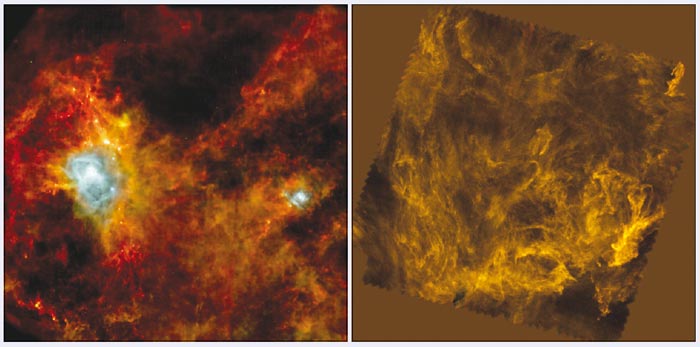
Indeed, Herschel has already taken a major step forward in showing how low-mass stars like the Sun were formed. Figure 3 shows pictures taken by Herschel of two of these stellar maternity wards, which exist as big clouds of gas and dust in a ring called the Gould Belt roughly centred on the Sun. Taken by a large international team led by Philippe André in Paris and including my colleagues in Cardiff, these pictures are actually pseudo-colour images made by combining three Herschel images taken at different wavelengths. The colours reveal the temperature of the dust, with red indicating cold dust and blue showing warm dust.
3 Blue is the colour The Herschel Space Observatory has been able to tell astronomers a lot about how low-mass stars like the Sun were formed. On the left, for example, is a sub-millimetre image of a cloud of dust and gas known as the Aquila Rift, created by combining three separate Herschel images. The colours indicate the temperature of the dust, with the blue regions being hot spots where the dust is heated by newly formed stars. A similar image of a different cloud known as the Polaris Flare, however, has only one colour, which indicates that its dust is all at exactly the same temperature and so has no newly formed stars. (Courtesy: ESA/SPIRE/PACS/P André for Gould Belt Survey; ESA/SPIRE/PACS/P André for Gould Belt Survey and A Abergel for EID Survey)
The picture of one of the clouds, the Aquila Rift, which is about 750 light-years from Earth, is a coruscating colour-drenched image that looks remarkably like a painting of a sunset on a stormy evening by William Turner in one of his more exuberant moods. The picture of the other cloud, the Polaris Flare, which is about 500 light-years away, is a monotonous brown. The explanation for the differences is that stars are being born in the Aquila Rift but not in the Polaris Flare. The full palette of colours for the Aquila Rift shows that the dust has a range of temperature, with the blue and yellow “paint drops” revealing warm spots heated by newly formed stars. In contrast with this Turneresque image, the monochrome image of the Polaris Flare shows that all the dust is at exactly the same temperature, and thus that there are no newly formed stars.
But why are stars being formed in one cloud but not the other? The answer appears to lie in the properties of the streaks of dust and gas, known as filaments, that snake across all the Herschel images of clouds in our galaxy, which can probably best be seen in the picture of the Polaris Flare. There appears to be a critical mass density of about five solar masses per light-year of filament length, above which – as in the Aquila Rift – gravity causes the filaments to collapse to form protostars that appear as beads on the filaments. Below the critical value, as in the Polaris Flare, the filaments never collapse and no stars are born.
But what causes the filaments to form in the first place? A clue appears to lie in the recent discovery by the Gould Belt team that while the density of the filaments can vary wildly, their width – no matter where they are seen in the galaxy – is always very similar, being about one third of a light-year. Remarkably, the team thinks it can explain this by turning to some simple physics of the turbulent interstellar gas. According to its model, the gas is usually flowing faster than the speed of sound in the gas, but when it slams into a big cloud of stationary gas, it slows down to below the speed of sound to form a filament. Indeed, the model says the gas piles up in exactly the way seen in the filaments.
This explanation is what simple physics suggests, but remember that astronomers are not working in a laboratory so it is rarely possible for us to “prove” anything. The best we can usually do is to find a model that fits our observations.
Another of astronomy’s big questions concerns how galaxies are formed. One of the big discoveries made 15 years ago with the first sub-millimetre camera on the JCMT was that there are some galaxies in the early universe that are so shrouded in dust that they are emitting 1000 times more radiation in the sub-millimetre waveband than at optical frequencies. Indeed, they are such luminous sub-millimetre sources that the dust must be hiding a very large number of newly formed stars. Calculations suggest that the stars are being created so quickly that an entire galaxy could be made in barely 100 million years, or about 1% of the age of the universe. These luminous sources therefore almost certainly hold a clue to how galaxies were formed.
The future is bright
Sub-millimetre astronomy is advancing at a quite astonishing pace. Just 15 years ago when astronomers started using the first sub-millimetre camera on the JCMT, it would take a whole night to find a single one of these shrouded galaxies. The top image above, which was the first taken by my team shortly after the Herschel Space Observatory was launched, took only 16 hours to make and reveals 7000 dusty galaxies – from those that are nearby to others that are so far out in space that we are looking 10 billion years back in time.
Unfortunately, the 2160 litres of liquid helium that Herschel originally contained will finally run out in March this year. When that happens, the cameras will warm up, and the telescope will become just another piece of space junk among millions of other bits of rubbish now floating in space. However, the treasure trove of Herschel data will be picked through by astronomers for years to come.
Meanwhile, a new sub-millimetre telescope – the Atacama Large Millimeter Array (ALMA) – has started operation 5000 m above sea level in the remote and inhospitable Atacama Desert in central Chile. Although ALMA can only operate in atmospheric windows at a few wavelengths, its advantage over Herschel is that it has much higher angular resolution. ALMA will therefore be able to produce detailed pictures of the galaxies that only appear as little blobs to Herschel. It is likely that ALMA’s observations of the sources detected in the Herschel surveys will be the key to providing answers to the origin of both stars and galaxies. William and Caroline Herschel would have been proud.