An alloy that undergoes a reversible temperature change of 31.5 K when squeezed has been created by physicists in China, Spain and the US. Materials that exhibit such a “colossal elastocaloric effect” could be used to create new types of highly-efficient refrigeration systems.
Refrigeration plays an important role in a wide range of human activity and keeping people and things cool consumes huge amounts of energy. Researchers are therefore very keen on developing alternatives to the relatively inefficient (about 20%) vapour compression systems that are in widespread use today. These refrigerators are also ripe for replacement because they tend to be noisy and use gases that can be dangerous or detrimental to the environment.
An alternative approach involves using “caloric” materials, which release heat when subjected to an external stimulus such as an applied magnetic or electric field or a compressive force. When the stimulus is removed, the material will absorb heat, thus cooling its surroundings. By applying and removing the stimulus on a carefully chosen timescale, a refrigeration cycle can be created.
In the past, much of the focus had been on creating refrigerators that use magnetocaloric materials. However, this has not led to the development of commercial devices for widespread use.
Low-cost option
Now, researchers are turning their attention to the elastocaloric effect, which involves squeezing solid crystalline (or polycrystalline) materials. Elastocaloric materials are attractive because they tend to have larger reversible temperature changes than magnetocalorics. They also tend to be less expensive – comprising alloys of metals rather than more pricy rare-earth magnets.
The elastocaloric effect occurs when a material undergoes a transition in its crystal structure when it is squeezed. This latest research was done by Daoyong Cong and colleagues at the University of Science and Technology in Beijing, the University of Barcelona and Argonne National Laboratory and focussed on an alloy of nickel, manganese and titanium (with a tiny amount of boron). The uncompressed material has an austenite crystal structure, that is converted to a martensite crystal structure by about 500 MPa of squeezing. This results in a change of temperature of 31.5 K. This is more than double the temperature change in the best magnetocaloric material and about 26% greater than the previous best elastocaloric – which is a nickel-manganese alloy.
The team used several criteria to select their elastocaloric material from a group of alloys containing nickel, manganese and one other metal. A material must undergo a large (about 2%) change in volume during the structural phase transition and the material must have mechanical properties that are compatible with being repeatedly squeezed and expanded. Furthermore, the material should be polycrystalline so that it can be easily and cheaply manufactured in bulk.
Writing in Physical Review Letters, the team describes their research as a “significant step forward towards large-scale elastocaloric refrigeration applications”. Furthermore, they say that their selection criteria could be used to find other materials that exhibit the colossal elastocaloric effect.
Since some sources of renewable energy are variable, at times power generators may produce output that is not needed. In the absence of energy storage systems, the surplus may have to be dumped or the power plant output turned down or switched off for a while. That may also have to happen if the grid cannot handle the power. Either way it is called “curtailment”.
Some specific reasons for curtailment include:
Weak grids: there may be congestion on the grid, especially local grids, making it hard for local projects to feed power to users when other projects are also employing the grid
Inflexible capacity: there may be large inflexible plants on the grid, e.g. nuclear plants, that cannot be turned down to allow use of power from variable renewables when it’s available
Over-capacity: it is likely that, in order to be able to meet average demand with variable renewables, more renewable capacity will be installed than is needed when demand is lower
Growing curtailment
In each case, the result can be wasteful: the potential output is not used. In recent years, the scale of this curtailment has grown; in some countries it’s become quite significant. For example, in China, where grid upgrades have not kept pace with the rapid expansion of wind energy generation, 20% of potential wind output was curtailed in 2016. China has been trying to deal with it, as I’ve noted in earlier posts.
In the UK, with well-developed grids, the problem is smaller. Indeed, the Policy Exchange puts the loss from wind in 2017 at just 1.5 TWh of wind, representing 0.4% of total UK power demand. Even output is sometimes being curtailed, which is wasteful environmentally and economically. Wind power companies, like most generation companies, have negotiated contracts to protect themselves from this. They get compensation payments, so-called “constraint payments” for power not generated or used. So far, the payments to wind projects have been a small proportion of the total constraint payments given to generators as a whole. They can nevertheless be provocative and, as wind and other renewables expand, the proportion will grow unless measures are taken to improve grids and balancing, including the provision of storage.
Some argue that curtailment is nothing new and does not matter — we have always accepted that some plants will have to be idle some of the time when demand is low. Indeed, in the case of fossil-fired plants, where fuel costs make up a significant part of the generation cost, not using them for a while will save money, although that has to be set against, on one hand, the loss of earnings and on the other, the avoidance of emissions.
However, with renewables like wind and photovoltaics (PV), where the fuel costs and emissions are zero, the balance is much more in favour of using the plant whenever possible, to earn income to pay off the construction costs. So curtailment should be avoided, although not if that involves excessive cost, e.g. for storage or grid upgrades: in some situations, curtailment may be the cheapest option. That will clearly often be the case if constraint payments are available. Some even say that in any case, with renewable costs falling we can afford to accept curtailment and build more capacity regardless. I will be looking at that contention in detail in a future post. For now, suffice it to say that the benefit may not be so clear if the value of the green energy forgone is high — it’s still a waste.
Negative prices
It’s a market-based issue. What’s more, curtailment, constraint payments or storage are not the only possible outcomes or options. There are other market responses and issues. Given the low marginal generation costs for renewable projects, if grid congestion is not the issue, the surplus output may sometimes simply be dumped on the power market at very low or even zero cost, possibly below retail or wholesale prices. That has been the case in Germany at times, and it’s been happening in the US too. Negative pricing has spread quite widely, including to the UK.
It can be good for consumers but not so good, economically, for renewable plant operators. This is part of a wider “race to the bottom” problem: as prices fall, there is less income available to support investment in new generation. More immediately, the fossil generators on the grid, for example gas turbines, cannot compete with these low marginal cost technologies and zero or even negative prices. If these gas plants abandon the market, as is a risk in Germany, that can have significant systems implications — there will be less capacity available when renewable inputs are low. That’s why capacity markets, or similar mechanisms, are being developed, to ensure that there is enough balancing capacity, in effect providing a subsidy to keep gas plants available or for other balancing services.
Surplus solutions
The simple message from this brief look at curtailment and system problems is that if renewables are to expand, there is a need to develop full grid-balancing capacity so as to avoid shortfalls, oversupply at other times and system conflicts. There is a positive potential outcome, however. If, rather than curtailing the occasional surplus output, this essentially free energy is stored and used to meet shortfalls at other times, then the problem of renewable supply variability has been at least partly solved.
Trading the surplus with other areas that have shortfalls is also an option, assuming the necessary long-distance grid transmission infrastructure has been developed. That can be used to import surpluses from elsewhere, if available when needed. For areas with regular surpluses, this could be a lucrative net trade.
It’s also possible to operate on the demand side, for example by pricing signals, so that peak demands are shifted to times when otherwise there may be low demand, too much power and a need for curtailment. In addition, on the heat demand side, some of the power surplus can be used to warm large heat stores – through immersion heaters in insulated water tanks, or other bulk heat store options, linking up with flexible combined heat and power (CHP) generation and heat networks. So variable power supplies can be used to meet varying heat demand.
Although establishing these measures will have costs, they may reduce overall system running costs, including curtailment costs, and help ensure the full balancing of variable renewables 24/7/365.
So curtailment can be dealt with, by improving grids but also by using the surpluses, and operating the power and pricing system in different ways. As we heard earlier, some think curtailment may in any case not be a major problem. A review by the UKERC found that curtailment can remain “at a low level even at very high penetrations of intermittent renewables”. It noted that “the point at which curtailment becomes significant can vary dramatically, with some analyses finding the inflection point to be as low as a 15% penetration and others finding the inflection point not being reached until there is over a 75% penetration of variable renewable generation”.
Broadly, UKERC says “the findings for relatively early curtailment are from studies focused on US electricity systems, with UK and European analyses suggesting that curtailment levels are very low until over 50% of electricity is supplied from variable renewables”.
It added “some level of curtailment may be both economically rational and sensible from a system operation perspective — so, in isolation, a degree of curtailment is not necessarily an indicator of the unsuitability of any particular form of variable renewable generation”.
That may be optimistic but although, perversely, low prices may be a problem as they make it hard for suppliers to earn enough to invest in new capacity, curtailment needn’t be a show stopper. It can be dealt with and doing so may open up interesting possibilities and net overall benefits, as long as there are not large inflexible plants on the grid making flexible balancing hard.
That was one of the messages in my 2016 IOP Publishing book Balancing Green Power [Editor’s note: IOP Publishing is the parent company of Physics World]. It is explored further in the revised and expanded version of my 2013 IOP Publishing book Renewables, which will be out soon. In my next post I look at what China is doing to reduce curtailment problems.
But can I end with a tribute to Professor Godfrey Boyle, a friend, Open University colleague and pioneer in renewables, who sadly has just died. Curtailed much too soon…
Researchers in the US have created a human blood–brain barrier (BBB) on a chip by recreating the development of brain microvascular capillaries in the embryo. The breakthrough could be used to develop more effective drugs and to better treat brain diseases (Nature Commun. 10.1038/s41467-019-10588-0).
The BBB’s primary primal role is to regulate access to the brain: it lets in the essential nutrients and energy metabolites required for good functioning of the brain while keeping toxins and pathogens at bay. Unfortunately, those substances that the brain staves off include potential life-saving drugs that could treat neurodegenerative disorders such as Alzheimer’s or Parkinson’s disease. For this reason, transient and localized opening of the BBB is one of the most researched and promising areas for emerging therapies that target the brain.
So far, studies have mainly resorted to animals such as mice or in vitro models to investigate the BBB and drug transport across it. But while these led to early breakthroughs in the field, they are not realistic enough to mimic the high functionality and complexity of the human barrier. Hence their use for development of drug and antibody shuttles that can cross the BBB is limited.
Culturing pluripotent stem cells under hypoxia
To solve this problem, Donald Ingber and his team from the Wyss Institute at Harvard University decided to upgrade one of their microfluidic organ-on-a-chip models of the BBB. Normally, the sealing of the BBB is assured by superposed layers composed of brain microvascular endothelial cells (BMVECs), adjacent multifunctional cells known as pericytes and non-neural brain cells called astrocytes. Instead of directly inserting adult cells in the two parallel channels of a chip, the team used induced pluripotent stem (iPS) cell technology and turned to physiology for inspiration.
Noticing that the BBB forms in the embryo with low-level oxygen (hypoxia), the researchers decided to culture the human iPS cells for an extended time in an atmosphere with only 5% oxygen concentration, instead of the normal 20%. Under these conditions, iPS cells developed into BMVECs that exhibited much more in vivo-like BBB properties than those grown under normal oxygen conditions.
These hypoxia-enhanced cells were subsequently cultured in one of the channels of a 2-channel microfluidic organ-on-a-chip device, while the other one was lined with human brain pericytes and astrocytes.
In vitro testing and drug development
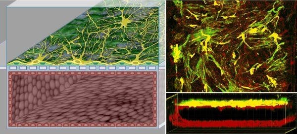
The two channels in the device are separated by a porous membrane. The channel lined with BMVECs is irrigated with a blood-like fluid at a physiological level of shear stress, while the other channel is perfused with a fluid that mimics cerebral spinal fluid. After three days of microfluidic cultures, the BMVECs had formed a tight monolayer with high barrier properties and had established connections with surrounding pericytes and astrocytes through the pores in the membrane.
The human BBB recreated in vitro in this manner was two orders of magnitude tighter than those previously generated without hypoxia or fluid shear stress, or past culture models with endothelium derived from adult brain instead of iPS cells.
BMVECs form a microvessel by covering all four sides of the lower of two parallel microfluidic channels (lower images), while pericytes and astrocytes populating the upper channel connect to the microvessel across a dividing porous membrane. (Courtesy: Wyss Institute at Harvard University)
More importantly, the engineered BBB contained a higher number of the selective transport and drug shuttle systems that are known to be present in the human BBB in vivo. The team tested the chip by injecting drugs and substances used in the clinic to treat brain diseases. For example, an increasing concentration of a mannitol solute temporally opened the BBB to allow the passage of large drugs like the anti-cancer antibody cetuximab.
These experiments highlighted the ability for the hypoxia-enhanced human BBB chip to selectively either prevent drugs from reaching their targets in the brain or allow transport of nutrients and drugs across the BBB.
The chip could be used for drug development studies and to model aspects of brain diseases that affect the BBB such as Alzheimer’s and Parkinson’s disease. It also opens the gate to advanced personalized medicine approaches by using patient-derived iPS cells.
As I’m sure you’ll have noticed, this month Physics World is celebrating the 50th anniversary of Neil Armstrong setting foot on the Moon for the first time. But what I’m interested in is whether we can commercialize the Moon or use it as a “space port” to take us further afield. At first sight, that might seem mad. Space is only 100 km away, but it’s an unforgiving place, where you need to have every bit of physics, maths and engineering right to make progress.
What’s more, getting to space – and staying there – is expensive. In 2015 an Atlas V rocket launched 8123 kg into low-Earth orbit at a cost of $164m – that’s more than $20,000 per kilogram. As the joke goes: escape velocity, you can’t leave home without it. So why, apart from proving its technical prowess, why would any business bother going to the Moon? Surely it doesn’t make commercial sense?
However, as I mentioned recently, getting into orbit is gradually becoming cheaper thanks in part to the reusable rocket technology developed by former physicist Elon Musk’s firm SpaceX. Its Falcon Heavy rocket can now get 53 tonnes into low-Earth orbit for $90m – that’s barely $1700 per kg. As the European Space Agency astronaut Tim Peake has said, firms like SpaceX are “forcing technology and industry” to compete, thereby “reducing the cost of entry” to space.
Private fortunes
Another boost to space innovation has come from tech giant Google, which in 2007 began funding the Lunar X Prize organized by the US-based X Prize Foundation. Worth $30m, the prize was earmarked for the first privately funded teams to land a robotic spacecraft on the Moon, travel 500 m and transmit high-definition video and images back to Earth. Five outfits were in the running for the award, although it eventually went unclaimed after the X Prize Foundation declared that “no team would be able to make a launch attempt to reach the Moon by the deadline [of 31 March 2018]”.
Nevertheless, one of the entrants – the Israeli non-profit organization SpaceIL – continued with its efforts and this February launched a craft to the Moon. Although its craft crash-landed on 11 April, SpaceIL was given a $1m “Moonshot Award” by the X Prize Foundation in recognition of the vehicle touching the surface of the Moon, which was still an amazing achievement.
So you want to be a trillionnaire?
But perhaps it really takes governments and national pride to fund projects that are so far from being commercially viable. China certainly thinks so. It recently landed the first spacecraft on the far side of the Moon as part of its Chang’e programme (see “Exploring the far side”). The US is also accelerating its Moon efforts, with NASA boss Jim Bridenstine recently announcing that Donald Trump wants to return to the Moon and to land humans on the surface again by 2024.
Bridenstine has promised “innovative new technologies and systems” to explore more locations across the surface than was ever thought possible. “This time, when we go to the Moon, we will stay,” he promised. “And then we will use what we learn on the Moon to take the next giant leap – sending astronauts to Mars.” But there’s also a clear commercial angle too as one aim of the programme is to develop a “space economy built on mining, tourism, and scientific research that will power and empower future generations”.
X Prize founder Peter Diamandis has even predicted that the world’s first “trillionaires” will make their riches from space – not from the Moon, but from asteroids. Although one Caltech study has put the cost of an asteroid-mining mission at an eye-popping $2.6bn, remember that building a rare-earth-metal mine on our planet is roughly $1bn. Given that a football-pitch-sized asteroid could contain as much as $50bn of platinum, you can see Diamandis’s thinking.
Mining an asteroid won’t be easy. Somehow, you need to get the raw material from the asteroid, through the Earth’s atmosphere and land it without destroying our planet. And even if you can bring the stuff home, the price for the platinum could plummet if supply outstrips demand. If I were a space entrepreneur, I’d probably not bother mining asteroids unless I could find something unique and valuable enough to warrant the effort or I needed the material in space, not on Earth.
Consider water. It currently costs up to $43,000 to send a bottle of water into space, which is why it’s all recycled on the International Space Station. But there are asteroids rich in water – so if you could mine it, you could split the water into hydrogen and oxygen, which would serve as fuel and oxidizer respectively. You could even set up “fuel stations” in low-Earth orbit and the asteroid belt so that spacecraft could fill up en route to the outer planets of the solar system. About 90% of the mass of a modern rocket is fuel, so carrying less on take-off would make space flight much more affordable.
We could build a number of small robotic Moon bases to mine ice
But rather than dragging a water-rich asteroid all the way back to Earth, it may be cheaper to make rocket fuel on the Moon. Indeed, NASA’s lunar-survey missions have already found lots of ice in permanently shadowed craters on the Moon. We could even build a number of small robotic Moon bases. Each would mine ice, make liquid propellant and transfer it to passing spacecraft. Perhaps the first true commercial opportunity for the Moon will be as our first interplanetary fuel station. And wouldn’t it be great if the world’s first trillionaire were a physicist reading this issue?
In the late 1970s the Dead Sea began to grow more saline as the rivers that fed it were diverted. And since 1979, crystals of salt have precipitated near the top of the lake and “snowed” down to the lakebed. The layer of salt in the deepest part of the lake thickens by about 10 cm each year but until now the way the crystals form wasn’t clear.
In summer the Sun warms and partly evaporates the top layer of water in the Dead Sea, making it even saltier. The salt snow originates here but the warmer, less dense water around it doesn’t mix with the colder water below. So how the salt was raining down into this colder layer was a puzzle.
In 2016 Nadav Lensky of the Geological Survey of Israel and colleagues took measurements at the Dead Sea and proposed an explanation — “double-diffusive salt fingers”. Now simulations by Lensky, Ouillon and colleagues indicate that this mechanism is correct.
“Initially you form these tiny fingers that are too small to observe… but quickly they interact with each other as they move down, and form larger and larger structures,” says Ouillon.
“The initial fingers might only be a few millimetres or a couple of centimetres thick, but they’re everywhere across the entire surface of the lake,” adds Eckart Meiburg, also of UC Santa Barbara. “Together these small fingers generate a tremendous amount of salt flux.”
The salt fingers form following small disturbances in the water, the researchers believe. Small parcels of warm water enter the colder water below and cool rapidly; heat diffuses faster than salt. Once it’s cooler the parcel can hold less salt and the salt precipitates out, forming crystals that sink to the lakebed.
The team’s simulations correctly predicted the downward flow of salt snow and the build-up of salt layers in the middle of the lake floor.
Salt crust
The finding could also explain other salt deposits. “We know that many places around the world have thick salt deposits in the Earth’s crust, and these deposits can be up to a kilometre thick,” says Meiburg. “But we’re uncertain how these salt deposits were generated throughout geological history.”
About six million years ago, the Strait of Gibraltar closed off, turning the Mediterranean into a shallow inland sea. Over several hundred thousand years the sea partly dried out, leaving salt deposits. The team’s discovery suggests that these deposits formed the same way as those in the Dead Sea. When the Strait of Gibraltar re-opened, water flooded the basin and sediment covered the salt.
The Moon has serenely and inexorably circled the Earth for millennia. Humans have regarded this glinting, mysterious object as both a source of wonder and as a fundamental landmark in the universe. The ancient Greeks even believed there was a sphere carrying the Moon that was the demarcation between our ever-changing, sublunary world and the incorruptible, unchanging and regularly moving heavens.
However, our relationship with our nearest neighbour has never altered so fast as it did after US President John F Kennedy spoke to the US Congress on Thursday 25 May 1961, a speech in which he committed his country to landing a human on the Moon by the end of the decade. It was a bold vision that was fulfilled on Sunday 20 July 1969 when Apollo 11’s Eagle lander touched down in the Sea of Tranquillity and Neil Armstrong took those first, faltering footsteps on the Moon.
The landing was a remarkable feat, watched by an estimated TV audience of 600 million, with Apollo 11 seeming to encapsulate the Zeitgeist of the age. Any scientific and technological challenge, no matter how grand, was surmountable if enough resources and expertise were devoted to it. Space was the new frontier – and science and technology would change the world for the better. Even today, the image of Buzz Aldrin in a white spacesuit, with a piercing black shadow cast on the lunar floor and Armstrong visible in the visor, remains iconic.
But the Apollo 11 mission did not just push human technology, engineering and endeavour to the limit. It also had science on board (see “Giant leaps for knowledge”). In particular, there was an ambitious experiment to install mirrors on the lunar surface. If light emitted by Earth-bound telescopes could be made to bounce off those surfaces, it would reveal the precise distance between the Earth and Moon. Previous studies using radar had shown the distance to be about 385,000 km (depending on the Moon’s orbital position) with an error bar of ±1 km.
Designed to improve on that measurement of the Earth–Moon distance, the Apollo 11 experiment duly fulfilled its goal. In fact, it became known as NASA’s most cost-effective experiment. But why, half a century on, are the results still challenging physicists?
Eagle’s egg
The roots of the new method for measuring the distance to the Moon originated in the late 1950s when Princeton University physicist Robert H Dicke, along with his collaborators and students, imagined mounting mirrors onto satellites. If they could bounce light off those on-board mirrors, researchers could not only precisely determine the orbital characteristics of the craft, but also obtain various fundamental scientific insights. These included tests of general relativity, and measurements of whether the gravitational constant G is not fixed but changes over time, which would be manifested by variations in the satellites’ orbits.
Shortly after Kennedy’s 1961 speech, Dicke’s students hatched a scheme to have spacecraft plant arrays of mirrors on the Moon. With the laser having been invented the year before (1960), they figured it might be possible to direct laser light off such an array and have the return light be detected by an Earth-based telescope. The time taken for the light to do the round trip – the “range” – would measure twice the distance between the telescope on the Earth and the array on the Moon. That in turn could be used to test general relativity and search for possible variations in G.
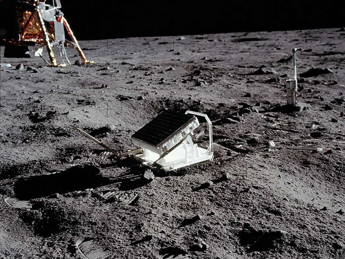
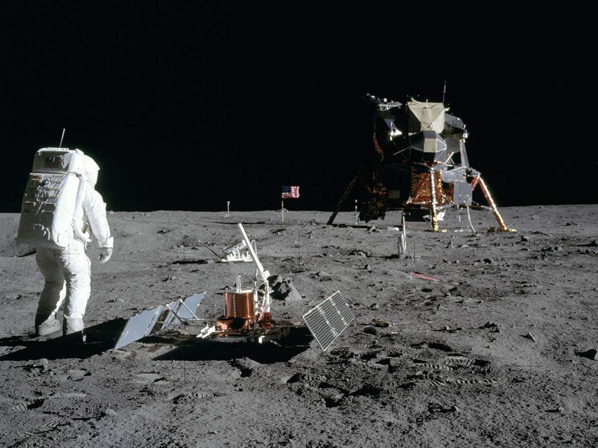
Measurement time: (above) Buzz Aldrin deploying the Early Apollo Scientific Experiments Package on 21 July 1969. In the foreground is the Passive Seismic Experiment Package; beyond it is the retroreflector for the Lunar Laser Ranging Experiment, designed to measure the distance from the Earth to the Moon. (Courtesy: Neil Armstrong/NASA)
In 1965 a group of Dicke’s students approached NASA with the idea for a lunar laser ranging (LLR) effort. Endorsed in principle two years later, the students then set up the Lunar Laser Ranging Experiment (LURE) team to carry out the project. LURE initially consisted of 10 experimental physicists, but the team quickly had to bring in experts on the orbits of the Moon and planets. “We realized we couldn’t just pick that up ourselves,” says James Faller, now 85, who had been one of Dicke’s graduate students at Princeton and was then at Wesleyan University. “It’s an art form that you don’t evolve in three months.”
We realized we couldn’t just pick [LURE] up ourselves. It’s an art form that you don’t evolve in three months.
James Faller
However, the Apollo spacecraft had room for only a small amount of science. Featuring a seismometer, a magnetometer, a suprathermal ion detector, a cold cathode gauge and a solar-wind spectrometer, the craft’s Apollo Lunar Scientific Experiments Package (ALSEP) had long been fully booked. It seemed as if LURE was not going to make the cut for that crucial first Moon landing. But then, in the autumn of 1968 and with little more than six months to go before the Apollo 11 launch date, NASA engineers decided to scale back how much cargo it could carry.
In seeking to minimize the time the astronauts would have to work on the lunar surface – for nobody knew how safe that would be – Apollo 11’s experimental package had to be entirely redesigned and simplified. Renamed the Early Apollo Scientific Experiments Package (EASEP), it now included less complex versions of the seismic, solar-wind and dust-detector instruments. Crucially, however, there was now room for LURE, which had the attraction of being quick and easy to install.
All the astronauts had to do was to carry the LLR device out, set it down on the lunar surface and orient it. The instrument was simple, reliable and low-maintenance. It had no moving parts and promised numerous scientific returns. The only concern was whether Eagle would stir up dust or kick off pieces of the module as it lifted up from the Moon’s surface on its journey back to the orbiting Columbia module. If dust or debris landed on the LLR device, the experiment would be ruined.
It was a risk the engineers decided to take.
Pressure mounts
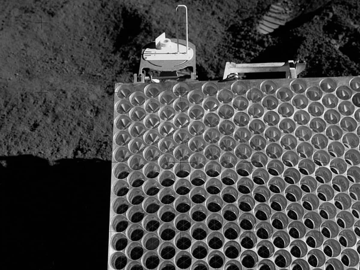
And so when the Eagle touched down on the Moon’s surface on 20 July 1969 – about 6 km from the expected landing point as the astronauts sought a smooth area to land – its cargo included a honeycomb array of 100 silica “corner cubes” measuring 46 × 46 cm in size. Each corner cube is an optical prism with three perpendicular reflecting faces – rather like three square mirrors joined at a single vertex. Together, they make incoming beams of light exit in exactly the opposite direction from which they entered (see box below).
On 21 July 1969 Armstrong and Aldrin placed this device, also known as a retroreflector, on the surface of the Moon, not far from the lander. Over the following years, four other arrays were installed too. Two slightly larger devices were placed by subsequent Apollo missions (14 and 15) in 1971, while two French-designed arrays were installed by Soviet lunar rovers in 1970 and 1973. However, the opportunity to place LURE aboard Apollo 11 had arisen so suddenly that no terrestrial telescopes were prepared to make observations.
Bigger, brighter, better: Consisting of an array of corner-cube mirrors, the Lunar Laser Ranging Experiment from Apollo 15 is currently the largest of four such devices on the Moon. A new design of retroreflector is currently scheduled to go to the Moon in 2020. (Courtesy: D Scott/NASA)
A ranging telescope would have to be able to direct a laser beam at the retroreflector’s location and then detect the photons on their return, which was not easy. What’s more, most existing telescopes were fully booked up with other observations. But NASA urgently wanted to be sure the ranging idea could be tested while the astronauts were still on the Moon’s surface so it would know the experiment worked, Suddenly members of the LURE team were under enormous pressure to find a telescope that could do so.
The Lick Observatory in California was one option, but it was available only for about two weeks because of other astronomical commitments. Keen to have a backup in case the weather at the Lick turned cloudy, and with only four months remaining before launch, the LURE team approached Harlan Smith, director of the McDonald Observatory in Texas. McDonald had a new, NASA-funded 2.7 m telescope for observing the planets, but Smith agreed to a crash programme led by Doug Currie – another of Dicke’s former PhD students – to design and implement technology for a long-term LLR effort.
When the Eagle landed and the retroreflector was installed, the Lick Observatory was ready but McDonald was not. At the Lick, Faller tried to observe returning light pulses but with no success. One major problem was that no-one knew the exact co-ordinates of the Eagle on the Moon. “God didn’t put an X where the lander was,” says Faller. By the time the Eagle had taken off, astronomers at the Lick still hadn’t detected any signal. Then, on 1 August 1969, and with the allotted time on the observatory running out, Dicke dropped in for a visit, grilling Faller about the equipment.
God didn’t put an X where the lander was.
James Faller
That night, 11 days after the Apollo 11 landing, they saw a signal – the first bounce of a laser pulse off the lunar surface. Dicke would later refer to it as a high point of his career. On 19 August 1969 the McDonald LLR facility – operated by Carroll Alley, another former Dicke student – made its first observation, and that observatory became the LURE project’s chief data-taker from 1970 for a decade and a half. Further measurements were made from the mid-1980s onwards by researchers at the Côte d’Azur Observatory in France.
But once LURE began to measure the Earth–Moon distance with centimetre rather than kilometre resolution, a host of new factors influencing that result came into play, all of which needed to be considered if astronomers were to properly understand their measurements. Shortly after the Apollo 11 mission, Jim Williams and colleagues at the Jet Propulsion Laboratory (JPL) in Pasadena, California, therefore started putting together a model to incorporate the principal factors affecting the lunar distance. It is a model they have been improving ever since.
Williams, who is now 78 but still works part-time at the JPL, ticked off a few of the factors that affect the Earth–Moon distance when I spoke to him recently. They include the orbits and orientations of the Earth and Moon, their rotations and wobbles, and their internal forces and structure. Then there’s the size and co-ordinates of the planets and major asteroids, plus perturbations from the Sun.
The analysis has to combine elements of physics, astronomy and geophysics.
Jim Williams, Jet Propulsion Laboratory
All told, the model has about 140 parameters, Williams explained. “But it leaves out some, and there may be others,” he admits. And all of these factors had to be incorporated into a model before the lunar distance could become a meaningful measure. The analysis has to combine elements of physics, astronomy and geophysics. “It has required me to learn new things,” Williams says.
How lunar laser ranging works
Lunar laser ranging, which measures the distance between the Earth and the Moon, is simple in principle. It involves an observatory using a powerful laser to target a series of short light pulses at an array of “corner cubes” placed on the Moon. Each cube has three perpendicular reflecting faces that make the incoming light exit in exactly the opposite direction from which it entered. Peer into a corner cube and you’ll see your eye’s iris in the centre, but – unlike in a mirror – your iris will stay dead centre even when you move your head.
Astronomers typically fire 20 bursts of light every second for between three and 10 minutes, carefully timing when each burst departs. The beam is initially as wide as the telescope’s mirror – about 3 m – but each pulse spreads out in transit due to diffraction and atmospheric turbulence. By the time it reaches the Moon’s surface about 385,000 km away, the pulse is shaped like a thin pancake about 2 km in diameter. The intensity is now so weak that only a trillionth of the photons in each pancake strike the retroreflector array.
After bouncing off the corner cubes, the photons return in exactly the reverse direction, also spreading out on the journey back to Earth. By the time they have come home, the signal is fainter still. Indeed, depending on the observatory, only one return photon is detected for every outbound shot. Still, that signal is just enough to be picked up by the originating telescope, amplified, and have its arrival time recorded. Knowing the speed of light, the distance to the Moon can be easily calculated.
On the rebound
Before LLR, the Moon’s distance from the Earth was known to within about a kilometre or so. Thanks to LLR, the resolution dropped to 20–30 cm in the mid-1970s, and to 2–3 cm by 2000. That year, in an attempt to reduce the uncertainty to about a millimetre, an ambitious project was mounted at the Apache Point Observatory in New Mexico. One of the central figures in this was the University of Washington physicist Tom Murphy, who was then just 29 and not even alive when the Apollo 11 astronauts installed the first array.
While finishing a PhD at the California Institute of Technology before getting a postdoc at the University of Washington, Murphy co-wrote a NASA proposal with two colleagues to use technologies that had not been used for LLR before, including avalanche photodiode arrays to amplify the signals. The project was called the Apache Point Observatory Lunar Laser-Ranging Operation (APOLLO), and it came online in 2005. “We thought we could improve the LLR measurement by an order of magnitude,” Murphy told me. “We were excited that we could make so many improvements in so many domains.”
It turned out to be much more challenging. For one thing, at the millimetre precision level, already-known influences had to be more carefully determined, and smaller influences that could be neglected at the centimetre resolution level now had to be included. “We ran into a rat’s nest of effects,” Murphy says. “We had to account for all the influences that affect the distance between the Earth telescope and the reflector sitting on the Moon to a new degree of sensitivity.”
We had to account for all the influences that affect the distance between the Earth telescope and the reflector sitting on the Moon to a new degree of sensitivity.
Tom Murphy, University of California, San Diego
Perturbations from the Sun can shift the lunar orbit by thousands of kilometres, while Venus and Jupiter each modify the Moon’s orbit by about a kilometre. That means Murphy’s team needed to know the locations and velocities of the planets to high precision, which is difficult. “There’s no stone tablet of the positions of all the bodies in the solar system – and each has unknown parameters, including 3D position, velocity and mass,” Murphy told me. “The uncertainty quickly adds up.”
The influence and location of all the heavenly bodies in the solar system was only one issue. At the millimetre resolution, knowing the exact co-ordinates of the terrestrial observatory and the lunar reflectors now became important too – and each of these is constantly in motion. “It’s eye-opening,” Murphy says. “You think the Earth is stable, but it all moves. The Earth’s crust is pushed by groundwater, by the atmosphere, by ocean loading – bodies of water in motion – and so forth.” Indeed, when tides pile up water on the California coast it literally moves New Mexico by a few millimetres. “Each site on the Earth and on the Moon has its own personality – its own unique displacements,” Murphy adds.
Much more information about the interior structures of both the Earth and Moon needed to be established and taken into account, which is why Murphy, who is now at the University of California, San Diego, is still working on the project almost 20 years on. But at the millimetre sensitivity level, even the mirrors on the Moon’s surface are no longer stable. Over the years, the performance of the retroreflectors has been ever so slightly reduced, evidently by dust kicked up every so often on the lunar surface. “I haven’t seen it, and I’m not 100% sure,” says Murphy, “but dust is the most economic explanation. Dust absorbs light and reduces the statistics.”
Still, the new resolution has allowed LLR to achieve many of its goals. One of the earliest concerned the equivalence principle, or the notion that inertial and gravitational masses are the same. If they were not identical, the different make-up of the Earth and the Moon would mean that the Sun could accelerate these two bodies at slightly different rates, which would affect the lunar orbit radius in a way that might be big enough to measure. No violation of the equivalence principle was seen. Nor was any evidence spotted for a variation in G, which indicated no increase or decrease in the lunar distance and period (2009 Int. J. Mod. Phys. D18 1129). The new resolution has, however, revealed much about the Moon’s interior, including the fact that it has some sort of fluid core – precisely what, though, remains unclear.
Currie – also still going strong – is among the leaders of an international group of scientists planning a Next Generation Lunar Retroreflector. It is scheduled to be carried to the lunar surface next summer by one of the commercial carriers now competing for NASA funding, and aims to improve the range accuracy by a factor of 30 and vastly expanding the scientific returns.
Contrasting legacies
Fine-tuned fundamental physical measurements are usually thought to give information about some feature of nature – the spin of the proton, the mass of the neutrino – that is disconnected, or largely so, from measures of other natural features. This is not true of the distance between the Earth and the Moon, which LLR has sought to measure. It cannot be worked out in a closed environment and is particularly intricate. Indeed, no matter how precise the instruments become, this intricacy will never go away and will become greater with each new measurement.
A close-up of the Apollo 11 Lunar Laser Ranging Experiment retroreflector. (Courtesy: NASA)
This new level of intricacy has also affected how the scientists involved have to work. Measuring the Earth–Moon distance requires collaborations between astronomers, astrophysicists and geophysicists, and between modellers and measurers. More and more detailed information about the positions, motions and even interior structures of all heavenly bodies have to be incorporated into understanding the meaning of each measure, while it is impossible to get a firm grip on all influences. These collaborations, too, will only get more complex still.
Fifty years on from the first Moon landing, the Apollo programme has left two strikingly different and contrasting legacies. One is the series of famous “Earthrise” photographs, starting with Apollo 8, which show a partly illuminated Earth poised just above the lunar horizon, as tranquil and implacable as the Moon seen from Earth (see image at top for the Apollo 11 Earthrise). The other, I would argue, is the LLR experiment, which is continuing to reveal ever more wobbling and juggling in the Earth and Moon, and the interaction of these two bodies with each other and with the other bodies in the solar system.
Philosophers often distinguish between “manifest” and “latent” images. The former is the world as described in the framework of ordinary human perception, while the latter is the world as described by the framework of science. Few things capture the difference better than the relation between the Earth and the Moon as depicted by “Earthrise” and by LLR. But for physicists, LLR’s many scientific returns are one reason why, 50 years after Apollo 11, it remains the only scientific instrument of that famous mission still in operation.
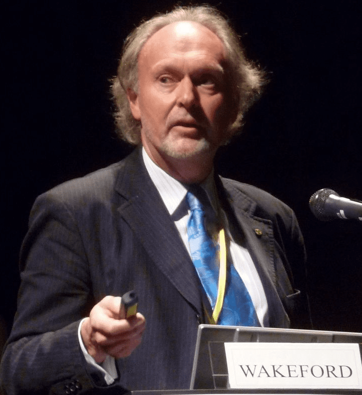
Radiation researcher: Richard Wakeford assesses the long-term impacts of radiation exposure (Courtesy: University of Manchester)
The Chernobyl disaster showed us that exposure to radiation can affect people to varying extents over different time scales, from acute radiation sickness to longer-term cancers. To take it back to basics, why does radiation harm us?
The health effects of radiation can be classed as two basic categories, usually these are referred to as deterministic and stochastic effects. Deterministic effects are high-dose effects, the sort produced close to an atomic explosion, or as a side effect of radiotherapy where high doses are involved, and the effects arise from cell killing. Radiation is actually a very good cell killer, hence the effect of radiotherapy on diseased cells. These acute effects, these deterministic effects, also affect healthy cells. If you kill off enough cells in an organ or tissue, it compromises its function and ultimately – as in the first responders of Chernobyl who got high enough whole-body doses – it kills them.
When you get down to lower dose levels, for example from natural background radiation or inhaling radon, then you do not get these cell-killing effects, because the levels of radiation exposure are not high enough. What you get are more subtle effects in the cell. These are modifications to the cell, conventionally of mutations in DNA. They do not kill the cell, but can lead to changes, such that in several years’ time this can develop into a cancer. Or if it is in a reproductive cell then a hereditary effect may occur in the descendants of the exposed individual.
You’ve written a lot about the challenges of picking out the impact of low-level radiation against the complex mix of other factors. Why is it so difficult to quantify the impacts of radiation exposure?
The basic problem boils down to this: there is not enough known about biology, and certainly not enough known about radiation biology. If it is a high enough dose, you know you are going to kill that person, or you are going to do some sort of damage to them. But at lower levels, then it is very tricky, and you do not know enough about radiation biology, so you fall back on epidemiology to derive risk estimates. Epidemiology involves looking at patterns of diseases in human populations to try and identify what might cause these patterns of diseases.
The big studies have involved the Japanese atomic bomb survivors. There, an enormous amount of effort has gone into following the health of approximately a hundred thousand survivors of the bombings of Hiroshima and Nagasaki in 1945, right up to now. It is still going on, because not all the survivors are dead. But in developed countries, perhaps between a third-and-a-half of everyone will develop some form of cancer at some time in their lives, for a number of reasons. If you are a smoker, for example, then the risk of lung cancer, and other cancers, goes right up because of the carcinogenic effects of inhalation of smoke. So, to extract a signal of lung cancer risk from exposure to radiation, let’s say in the bomb survivors, from the smoking pattern – and smoking dominates the risk of lung cancer – is a very tricky thing.
With those difficulties in mind, how do you assess the relative risk of exposure to low-level radiation?
You also get into the other noise of the background causes: genetic makeup, whether they take exercise, what they drink, what they eat. This background noise tends to be what dominates the overall risk of, let’s say cancer, and then the small additional risk arising from increased exposure to radiation is very difficult to pick out from this background noise. That is why there is still some uncertainty in just what level of risk there might be for everyday exposure to radiation, say if you go in to have a CT scan. We know it must be pretty low, otherwise the results of that exposure would be obvious for all to see, as it was for the highly exposed bomb survivors. But just what level there might be is more uncertain.
For the purposes of radiological protection, it is assumed that the increased risk is directly proportional to the dose of radiation that you have received, modified by certain factors, because we know that exposure of young people imposes more risk per unit dose than exposure of older people, and that women are more sensitive than men. That direct proportionality goes right the way down to the very lowest doses.
HBO’s recent TV series has reignited public interest in the 1986 disaster at the Chernobyl Nuclear Power Plant. What lessons did we learn from that disaster?
At Chernobyl, there were four units and it was Chernobyl Unit Four that exploded. These were rather unusual Soviet-style reactors, RBMK reactors, which were inherently unstable, and the operators were carrying out experiments on the reactor that they really should not have been doing. They were unauthorised experiments, and of course it led to the explosion of the reactor. I suppose one of the first lessons is what happened to the early responders, the first guys who had come to deal with all this exposed nuclear fuel on the ground; 134 of them suffered acute radiation syndrome because of the high doses that they had received and 28 of them died. Clearly now, if you can at all help it, you do not put people into those situations.
The next lesson to be learned there, which was applied for the more recent Fukushima accident in Japan, is that you have to move people out of harm’s way quickly, which they did not do after the Chernobyl accident. It took about 36 hours for people in the immediate vicinity of Chernobyl to be evacuated. While at the Fukushima Daiichi plant, as soon as it appeared that there were serious problems, they moved people out of an area of twenty kilometres in radius around the site just in case the worst happened.
How about the years since the Chernobyl accident – what have been the longer-term impacts and what have we learned?
The really bad thing, I guess, at Chernobyl is that children were allowed to continue to consume cow’s milk, which was heavily contaminated with radioactive iodine. Radioactive iodine concentrates in the thyroid gland, and it was already known before Chernobyl that children are particularly susceptible to an increased risk in the future of thyroid cancer. In the neighbourhood of Chernobyl, more than ten thousand children received thyroid doses in excess of one gray [J kg -1], which is more than a thousand times greater than you would receive in a year from natural background radiation. The consequences of that became apparent in the early 1990s, when relatively large numbers of thyroid cancers started to be detected in those who had been exposed as children, and that continues today. We have already seen thousands of additional cases of thyroid cancers, we can expect many more thousands of additional cases of thyroid cancers, as a consequence of that initial exposure to radioactive iodine. Fortunately, thyroid cancer is rarely fatal, because the thyroid gland can be removed, and so this exposure from Chernobyl has caused about fifty or so deaths so far, but that is out of several thousand thyroid cancer cases.
In Fukushima, they were of course aware of this. There was radioactive iodine released from Fukushima Daiichi. Fortunately, most of it went out to the east over the Pacific Ocean, but some of it did come back inland. The authorities were well aware of that, and certainly any contaminated milk was restricted from distribution. They were also aware of other contaminated food items. It looks like thyroid doses to children in Fukushima were very low, and certainly much lower than those received around Chernobyl.
The 30-kilometre exclusion zone around Chernobyl is still barely habited. While at Fukushima, some residents have started to return but some areas remain fully or partially restricted. In both cases, will some areas remain restricted indefinitely?
It will not be indefinite. If you take Chernobyl, for example, the principal contaminants there of concern were iodine-131, so that is the thing that caused much of problem of thyroid cancer – thyroid cancer among those that were exposed as children, to be exact. That has a half-life of eight days, so that is gone in 3 months, and then you have the radioisotopes of caesium, and these are the other volatiles that were emitted. So caesium-134 has a half-life of around two years, so that is essentially all gone now, and what is left there is caesium-137, which has a half-life of around thirty years, so that is much more of a protracted problem – it is called “groundshine”, the gamma radiation from caesium-137 that settled out in the environment. That is the principal problem in Fukushima, as well, and what is causing some of the areas that were evacuated after the accident at Fukushima to still be evacuated, and where resettlement has not been permitted.
But if you go back to some of these areas, then the environmental exposure to gamma radiation gives you a dose of fifty millisieverts or more per year, which compares with one or two millisieverts that you get from background radiation. At the moment, the Japanese authorities are working to a safety level of twenty millisieverts per year, to allow people to return. Exposure is falling away all the time, of course, through naturally occurring radioactive decay, but also through dilution in the environment – it is becoming buried, which shields the radiation. It is a problem. It will, of course, eventually go. In three hundred years, it is gone. But the question is what to do now for these settlements where there are still these high levels of contamination – pressure-hosing roofs, taking off top soil, these sorts of things. But it is very tricky, because this is a mountainous, forested area. If it rains, it brings down more contaminated soil from the mountain, so they have got a problem.
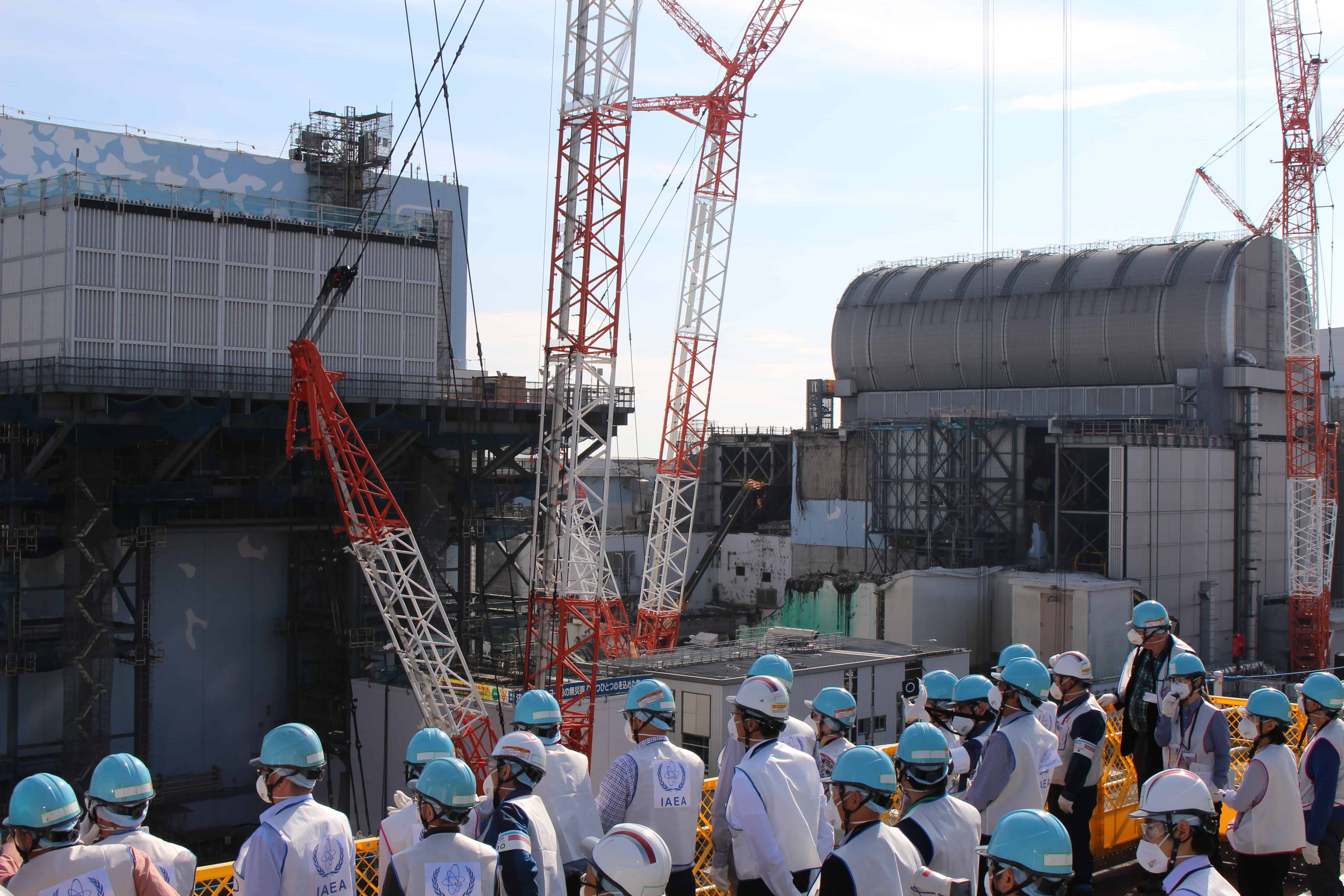
Site Inspection for IAEA Decommissioning Review Mission at Fukushima Daiichi NPS on 7 November 2018 (Courtesy: TEPCO)
You’ve written in one of your papers about the psycho-social effects of experiencing an event like Chernobyl, and how it can have a long term impact on your health beyond the radiation effects?
I do not think that there is any doubt that there is this disaster syndrome. I mean, those that were evacuated as a consequence of Chernobyl or Fukushima, for example, do have, undoubtedly, a psychological impact, purely by the fact that they had to be relocated, maybe permanently. Some of the Chernobyl evacuees, of course, still have not been permitted to return to the exclusion zone, although some of them have, unofficially. So yes, there is that impact, and others, including changes in lifestyle. In terms of cardiovascular disease, it is more a question of, again, what people do in the background. Do they smoke? Are they obese? What do they eat? What is their genetic makeup? In terms of their overall risk, and background risk of cardiovascular disease, to try and extract a small radiation signal against that background of effects is tremendously difficult.
Coming back to Chernobyl, for example, there has been a book published recently [Manual for Survival: A Chernobyl Guide to the Future by Kate Brown] suggesting that the risks to health of the Chernobyl accident have been dramatically underestimated by the expert committees that have looked at this. But distinguishing the effects of radiation exposure from Chernobyl against the health effects which arise from the collapse of the Soviet Union, which was quite dramatic, is a real problem. If you look at Russia, the age-adjusted mortality rate in Russia is like a rollercoaster, reflecting the socioeconomic chaos that resulted from the collapse of the Soviet Union. In the 1990s, the mortality rate rocketed.
To distinguish a Chernobyl signal from that background is immensely difficult, and this is right across Russia, an enormous country. If anything, these effects are even more marked around Vladivostok in the far east of the country. I think what has happened is that many people have associated these more general health effects that they have experienced across the old Soviet Union, with Chernobyl, when in fact these effects would have been there had the Chernobyl accident never happened. This is really a classic example of the difficulties of epidemiology, and how mistaken it can be to associate various health effects with one thing, when in fact it is a more general thing that is causing those effects.
In recent years, both the Chernobyl exclusion zone and the Fukushima disaster area have attracted visitors interested and there are now a number of tours. What is it about these events and places that creates such profound fascination among people?
I guess it is sort of disaster tourism, isn’t it, really? I guess these things have such a position in the public imagination that they need to see these places. I went to Fukushima Daiichi six months after the accident with an international group of scientists to look at the place and talk to people, and to see what was going to be done. I have to say, it was fascinating. You go down to the site, which is a big site – it was six reactors, three were operational at the time of the earthquake – and see the damage that was done by the fifteen-metre tsunami!
I guess, having been there, it is the fascination of seeing the place. I have never been to Chernobyl, but I can understand why: here is one of the big, iconic disasters, particularly a nuclear disaster, and there is this fascination with things – radiation, nuclear, and all the rest of it. People are just fascinated by going to see the place, I guess. It extends to everyone, essentially.
Fukushima had a big impact on the nuclear power industry, with nations reacting with varying degrees of concern. Do you think it has changed public perception on whether nuclear power is actually worth the risk?
It had an enormous impact on public perception and the nuclear power programmes in Germany and Switzerland were shut down as a consequence, principally, of the Fukushima accident. From what I see of the situation, Chernobyl was the worst nuclear accident that there has been, but I guess people sort of said, “Well, this was an accident involving a strange Soviet-style reactor, in the Soviet Union, which was on its last legs, which dissolved into the various countries four years later”.
Japan was more of a shock. I mean here is a technologically advanced country, and running these standard BWRs [boiling water reactors] at the Fukushima Daiichi site, and that was a bit of a shock, because the nuclear industry had this concept of “defence in depth”. Fortunately, the Japanese on the east coast of Japan were well aware of the problems of big earthquakes off the coast, and big tsunamis – these are about one in a century occurrences. But although they built a six-metre-high anti-tsunami wall, of course that fifteen-metre wave went straight over the top of it and did considerable damage to the plant. The real problem was that the external power lines had been brought down. So, the diesel generators started up, as they should have done, to keep emergency services like pumps running, but they were situated in the basements of buildings, so they were flooded by the tsunami, and they were knocked out.
If you have a site like Fukushima Daiichi, which was operational in the 1970s, so it had been going for forty years or so, you could not rule out a big tsunami occurring at some point during its operational lifetime. So, defence in depth had failed, and it had failed in a technologically advanced country, which had a large number of reactors.
So what now for safety in nuclear power plants? Have we learned anything new from Fukushima?
I would hope so. There are a large number of nuclear power stations, for example, being built in China now. In the UK, there’s one being built at Hinkley Point and some elsewhere in Europe, so you would like to think that the importance of defence in depth has really hit home to those countries that run nuclear reactors. And there is reason to believe that it has, from the “stress tests” that have been run by regulatory authorities on these facilities to see if nuclear plant safety regimes can meet these sorts of challenges – loss of power, and all the rest of it.
So, I would hope that organisations such as the International Atomic Energy Agency have reminded their members of the importance of defence in depth, and of checking these systems, and having a proper and independent regulatory system in place, which has “teeth” if they do find something that an operator is not doing right.
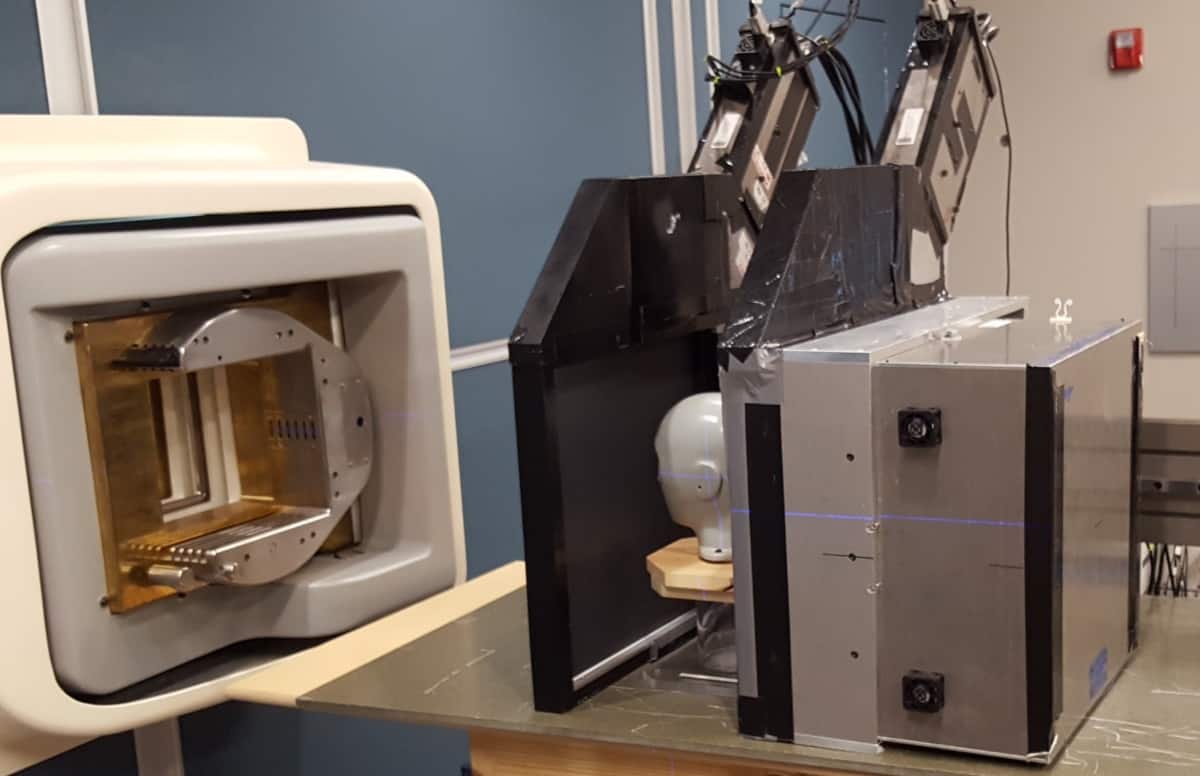
Proton radiography set-up showing the two 2D proton detectors on either side of the head phantom along with the residual energy detector. (Courtesy: James Welsh)
One major challenge when delivering proton therapy is uncertainty in the range of a clinical proton beam travelling through the various tissues and organs in the body. To address this problem, US researchers are developing a system for proton CT and radiography, which could be used both for image guidance and estimation of proton beam range in the clinic. They have now presented the first proton radiographs using their system, including the first real images of biological materials (J. Radiat. Oncol. 10.1007/s13566-019-00376-0).
Currently, proton therapy is planned using X-ray-based CT. The CT data are also used to create digitally reconstructed radiographs (DRRs) for use in daily patient set-up, by comparing the DRRs to X-ray images recorded immediately prior to treatment. This approach, however, introduces inherent inaccuracies due to the need to convert CT Hounsfield units into proton relative stopping power.
In analogy to the creation of DRRs, the proton CT data can also be used to generate proton DRRs. These pDRRs could someday replace X-rays for high-precision patient alignment in the daily image-guidance process, as well as providing proton range information. Notably, the estimated radiation dose to the patient is only around 1% of the absorbed dose delivered by the X-ray-based approach.
The team has developed a compact proton imaging set-up based on plastic fast scintillation 2D tracking detectors, which detect individual protons in two dimensions, and a photomultiplier tube-based residual range detector. The 2D proton detectors are placed proximal and distal to the patient, while the range detector is located beyond the distal tracking detector.
To assess their system, the researchers used the Geant4 Monte Carlo algorithm to create a series of pDRRs from patient X-ray CT data. Three physicians then evaluated the image quality of these idealized pDRRs. All three felt that the pDRRs showed sufficient anatomical detail for patient alignment.
“If the pDRRs were derived from proton CT data, the results would be very similar,” explains senior author James Welsh. “But the pDRRs from proton CT data would be more accurate, since the proton stopping power is measured directly.”
The researchers also obtained the first actual proton radiographs of a biological specimen using their system. Images of a frozen tilapia cichlid fish revealed the fish’s internal bony anatomy. The high level of detail suggests that human bony anatomy will be similarly evident using the system, with images useable for daily image-guidance. Welsh notes that the team has also recently obtained its first proton CT images.
Image reconstruction
In a separate publication, Welsh and colleagues present an image reconstruction system for the prototype proton radiography system. They used Geant4 to simulate raw data detected by the device and wrote dedicated software – pRad – to process these data and reconstruct radiographs (J. Radiat. Oncol. 10.1007/s13566-019-00387-x).
James Welsh (far left) and the research team. (Courtesy: James Welsh)
The researchers simulated proton pencil-beam irradiation of a paediatric head phantom. They used the pRad software to reconstruct proton radiographs showing the 2D distribution of water-equivalent path length (WEPL) values. Using a desktop computer with a single CPU and a single graphics processing unit, the software took about 11 s to reconstruct a radiograph from 7.6 million protons.
The team generated radiographs using an iterative reconstruction algorithm, plus two fast non-iterative methods – straight-line projection (SLP) binning and most-likely paths (MLP) binning – and compared the results with a “ground truth” image. They also compared three methods for defining the hull (the surface of the imaged object): one using the known geometry of the object, and two using WEPL to estimate the hull.
Most features in the ground truth image were visible in the reconstructed radiographs, with departures from truth mainly occurring near the outer edges of the object. Radiographs reconstructed with a known hull showed sharper outlines, while simple SLP binning gave the worst results, regardless of hull method used. In all iterative reconstruction and MLP binning cases, the mean WEPL error in the head phantom radiograph was less than 1 mm.
The researchers also simulated proton imaging with intentional misalignments (lateral shifts or rotations) and reconstructed the simulated data with and without alignment correction. The latter illustrated how bad reconstructions arise from misaligned data, while the former demonstrated the effectiveness of the alignment-correction algorithm.
“While there are many challenges with respect to both hardware and software, our prototype is clinically practical enough that we have been able to form a partnership with an interested industrial partner (Cosylab), with the goal of achieving integration into proton therapy treatment rooms,” Welsh tells Physics World. “We are now designing the clinical version and extending automatic image reconstruction to proton CT as well as proton radiography.”
Many of our everyday foods rely on pollinators but these animals – bees, butterflies, moths, beetles, birds, bats, rodents and even lizards – appear to be in decline. A new study sets out a strategy for pollinators that will help ensure we still have tomatoes, kiwi-fruit, runner-beans, apples, brazil nuts and courgettes on our plates.
Scientists have tracked population trends for a few hundred species of bee, mostly in temperate regions of northern Europe and North America. But more than 20,000 species have been identified and it’s near impossible to monitor them all.
“The ones to have been studied are often from iconic groups like bumblebees, which are big and colourful species,” says Ignasi Bartomeus from the Doñana Biological Station in Seville, Spain.
Long term data are lacking from many other parts of the world, leaving us somewhat in the dark as to how pollinators are faring.
From the early Victorian naturalists collecting insects in their own gardens, to the conservation volunteers of today, an army of citizens has been keeping watch for more than 100 years
Lynn Dicks
Nonetheless, we do know that pollinator decline is being driven by agricultural expansion, agricultural intensification, including increased use of pesticides, and climate change.
“We can predict that pollinator declines of the magnitude seen in Europe and North America are occurring in Asia and Latin America, and starting to occur in Africa, but we can’t test this prediction with scientific data at the moment,” says Lynn Dicks from the University of East Anglia, UK.
Together Bartomeus and Dicks identified the gaps in our knowledge concerning pollinators, investigated why those gaps exist, and looked at what needs to be done to conserve pollinators.
One of the main barriers the scientists identify is the difficulty of accessing historic data. In their paper in Environmental Research Letters (ERL) they write that one of the first actions needs to be “redoubling the efforts to make historical data on species occurrences, interactions and traits openly available and easy to integrate across databases”.
But the pair also believe that research culture and the way that funding is allocated need to change. “Researchers are usually rewarded for leading projects and generating new ideas, but less so for collaboration and monitoring,” says Bartomeus. “Upscaling and testing the generality of ideas and participating in large collaborations should be more valued to stimulate coordinated collaborations.”
When it comes to gathering data Bartomeus and Dicks envisage citizen scientists playing a major role. “All the standard monitoring and recording schemes that have provided long-term data for Europe and North America are run and conducted by volunteers,” says Dicks. “From the early Victorian naturalists collecting insects in their own gardens, to the conservation volunteers of today, an army of citizens has been keeping watch for more than 100 years.”
Finally, Bartomeus and Dicks believe that there needs to be a fundamental shift in research infrastructures, to allow integration of social, economic and ecological approaches, and to encourage collaboration between stakeholders, including scientists, managers, members of the public and farmers.
“As a community, it would be a huge step forward to create comparable protocols and experiments by consensus that can be adopted by any researcher or citizen science project and collected in central places,” they write.
The lithium-ion anode is the material of choice in battery applications thanks to its high specific capacity of 3.860 Ah/g and low electrochemical potential of –3.04 V. In practice, however, the performance of lithium falls far short of its theoretical potential because it has a low Coulombic (cycling) efficiency. Another reason is that it is incompatible with conventional electrolytes, which leads to needle-like dendrite formation on the anode surface during battery operation. As well as degrading battery efficiency and reducing battery life by creating a porous Li-metal structure that consumes both active Li and electrolyte, these dendrites can also create short circuits and in some cases, cause devices to explode.
Liquified gas electrolytes could help overcome this problem. These electrolytes, first reported on in 2017, are made, as their name suggests, from liquified gas solvents. They function at both room temperature and at very low temperatures (down to –60 °C) because they are more resistant to freezing than standard electrolytes.
Dendrite-free Li-metal cycling
Researchers at the University of California San Diego (UCSD) and the UCSD spin-off company South 8 Technologies led by Shirley Meng and Cyrus Rustomji studied the fluoromethane (CH3)-based liquified gas electrolyte. Previous work showed that this electrolyte allows for dendrite-free Li-metal cycling with a relatively high efficiency (of 97.5%) by forming a dense, uniform, ceramic-based solid-electrolyte interface (SEI) composed mainly of LiF and Li2CO3 salt on the Li anode surface. This SEI is different to the inhomogeneous SEI that forms with conventional electrolytes, which is unstable and produces dendrites.
In the previous work, researchers found that the cell performance of liquified gas electrolytes was limited because the lithium salt has limited solubility in the electrolyte , which leads to high polarizations. Meng and colleagues have now overcome this problem by adding small amounts of tetrahydrofuran as a co-solvent to the electrolyte. What is more, they say that they now fully understand the solvation structure and improved lithium transport in the electrolyte thanks to electrolytic conductivity measurements and molecular dynamics simulations.
Unlike typical electrolytes
For one, the conductivity versus temperature curves of the liquefied gas electrolytes do not follow that of typical electrolytes, they say. Because of the exceptionally low melting point of the fluoromethane, its minimal viscosity, and high dielectric-fluidity factor, the conductivity is well maintained at low temperatures. Indeed, the conductivity is considerably enhanced with an increase in concentration of the salt and additive while still following the same temperature trends as the fluoromethane-based electrolyte without the addition of tetrahydrofuran, explain the researchers.
“The unique properties and solvation structure of liquified gas electrolytes result not only in high overall conductivity but also in the unusually high contribution of the lithium cation to conduction that is highly desirable,” says team member Oleg Borodin of the Army Research Laboratory. “The fluoromethane-based liquid gas electrolytes containing additive amounts of tetrahydrofuran also fully coordinate with lithium cations and greatly enhance salt dissection and transport.”
The electrolyte also boasts a lithium transference number of more than 0.79, a low viscosity, low melting point and high dielectric fluidity factor, he tells Physics World. It also forms a stable F-rich SEI with the Li metal anode that has significantly lower resistance than traditional electrolytes.
Less than 1% porosity
The high transference number, low viscosity and stable SEI are key for lithium metal cycling, to prevent dendrite growth and allow for dense, smooth Li deposition. The researchers proved this by measuring the porosity of lithium deposition on the current collector in their battery using a cryogenic-focused ion beam and 3D reconstruction. The porosity with liquified gas electrolytes is just 0.90% at room temperature. To compare, this increases to nearly 17% with conventional electrolytes.
The low viscosity and melting point enable higher conductivity down to low temperatures, which results in impressive Li metal cycling efficiency at these temperatures – even at a high cycling rate. Indeed, the researchers found the cycling efficiency of the lithium-anode in their experiments was 99.6% for 500 charge cycles at room temperature. This is better than the 97.5% reported in 2017 and the 85% for the anodes in a conventional (liquid) electrolytes. At –60 °C, this value drops slightly to 98.4%. A feat in itself since most conventional electrolytes do not work below –20 °C.
Until now, researchers have mainly been studying high concentration liquid electrolyte or electrolyte systems for improving lithium-anodes, but liquified gas electrolytes could be more promising, say Meng and colleagues – especially for low-temperature operation applications.
“South 8 Technologies, is now commercializing this technology”, says team member Yangyuchen Yang. “Our research group is also focusing on better understanding these electrolytes and optimizing them based on both modelling and experimental studies.”



 Lunar laser ranging, which measures the distance between the Earth and the Moon, is simple in principle. It involves an observatory using a powerful laser to target a series of short light pulses at an array of “corner cubes” placed on the Moon. Each cube has three perpendicular reflecting faces that make the incoming light exit in exactly the opposite direction from which it entered. Peer into a corner cube and you’ll see your eye’s iris in the centre, but – unlike in a mirror – your iris will stay dead centre even when you move your head.