Page 893 – Physics World

Home » Page 893

Liquid mysteries

When I read scientific papers, I often end up pondering questions that are – in the grand scheme of things – mere footnotes and details. Quite simply, I lose sight of the big issues. Fortunately, one benefit of teaching physics to undergraduates, as I do, is that it lets me take a broader perspective. Take the way that textbooks deal with the fundamental differences between the states of matter. While these works contain neat and cohesive descriptions of gases and solids, many struggle with liquids.

Consider David Tabor’s classic book Gases, Liquids and Solids, which has been reprinted many times since it was first published in 1969. “The main characteristics of [the gaseous and solid states] are well understood,” Tabor writes. “By contrast the liquid state, in some ways, has ‘no right to exist’ [and] raises a number of very difficult theoretical problems.” Then there’s Franz Mandl’s 1971 book Statistical Physics, in which he discusses the qualitative differences between liquids and solids, but then throws in a disclaimer that his argument is “not accepted by everyone”.

As we can see, scientists’ confusion regarding the description of the liquid state has been bubbling beneath the surface for decades. But if you think we have a problem understanding liquids, the situation is even worse with the “supercritical fluid” state, which I’ll come to later. However, recent advances mean we could resolve these problems and provide theoretical descriptions of both the liquid and supercritical fluid states over the wide range of pressures and temperatures that they exist across.

Liquids – what a gas!

While some physicists have tried to describe the liquid state directly from first principles – that is to say, without referring to the solid or gas states – this approach is very difficult. In a crystalline solid, the high level of order makes calculations and computations relatively easy. In a gas, the lack of any structural order is used to simplify calculations and computation instead. However, to fully understand the liquid and supercritical fluid states, neither option can be used. Instead, what researchers usually do is to use gases as a starting point and make some adjustments.

One way to do this is to wheel out the Van der Waals equation of state. In this approach, a sample is described as a non-ideal gas, in which the particles have a specific size (rather than being infinitely small point masses) and there is an attractive Van der Waals force between them. By applying this equation to liquids, you can understand boiling as a “first-order” phase transition, which means that as it turns from liquid to gas, there is a discontinuous (rather than smooth) jump in the material’s properties, such as its density, heat capacity and entropy.

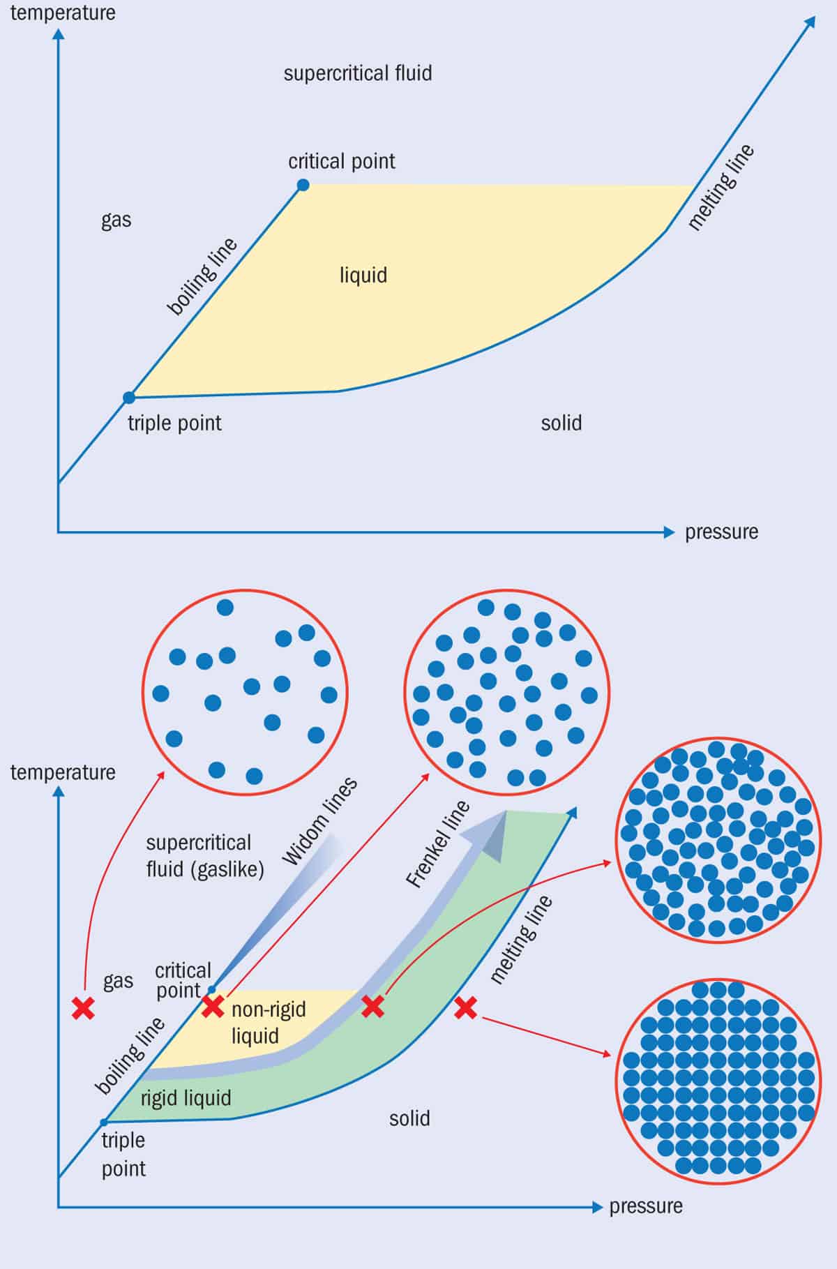
However, physicists are not interested only in what happens to a liquid at a single pressure. If you raise the pressure, the boiling temperature goes up too, with the line dividing the two states of matter on a temperature/pressure graph being known as the “boiling line” (figure 1a). What’s interesting is that as you go up in pressure, the jump in the liquid’s density, heat capacity and entropy as it boils becomes steadily smaller. Eventually, when the pressure is sufficiently high, a “critical point” is reached, beyond which there is no boiling transition at all. With no phase transition between liquid and gas states, the sample is now a supercritical fluid, a still-mysterious phase that shares properties of both a liquid and a gas.

Most textbooks leave liquids and supercritical fluids at that; but the supercritical fluid state has a complexity that physicists are only now starting to appreciate. For starters, parameters such as density, which usually change abruptly and discontinuously when we cross the boiling line, do something different if we make a transition above (albeit close to) the critical point. They still change over a narrow range of pressure or temperature but now do so continuously, not in a jump.

What this means is that the boiling line can now be extended beyond the critical point, where it is dubbed the “Widom line”, in honour of the Cornell University chemist Benjamin Widom (figure 1b). Indeed, we can plot out separate Widom lines for all the different properties that change when we boil a liquid, including its density, speed of sound and heat capacity. The Widom line links the different pressure-temperature points where there is a narrow change in each property. They start at the critical point but gradually diverge from each other and get smeared out.

Interestingly, if we increase the pressure on a liquid or supercritical fluid at a fixed temperature the sample always eventually solidifies. Nitrogen, for example, becomes a solid at room temperature if you squeeze it to about 24,000 bars pressure (2.4 × 10⁹ N/m²). Even hydrogen solidifies at room temperature if you take it to 55,000 bars. Using modern equipment, such as the diamond anvil cell, these kinds of experiments are routine; we really can take air from the atmosphere and freeze it solid.

Dean Smith from the University of Salford at the Diamond Light Source in the UK — The pressure mounts: Liquids can be routinely squeezed to high pressures using a diamond anvil cell. (Courtesy: John Proctor)

But the problem is that long before it solidifies, the fluid becomes so dense that we can no longer describe it as being similar to a gas. For instance, in dense molecular fluids, such as water, neighbouring molecules will slot together in an ordered manner over short distances almost exactly like they do in solids. What’s more, a variety of experiments dating back to the 1960s have shown that dense fluids support shear waves. Both types of behaviour are totally different to what is observed in gases and in liquids near the critical point.

A solid start

As it is hard to describe these kinds of liquids and fluids by starting off with the behaviour of a gas, some physicists have instead tried to liken them to solids. Various theoretical descriptions of this ilk have been put forward over the decades or, if you include Maxwell’s work, over the centuries. Based on this solid-based approach, researchers have recently been able to model properties of dense fluids, discovering that they take on certain solid-like properties as you raise the pressure (P) or lower the temperature (T). Surprisingly, the onset of these properties occurs within a relatively narrow P–T range.

This narrow P–T range has been named the “Frenkel line” (figure 1b) after the Soviet physicist Yakov Ilyich Frenkel (1894–1952), who pioneered the solid-like theoretical approach to liquids. But what do we know about liquids beyond the Frenkel line? At the critical point, there is just enough room to squeeze in an additional particle in-between two adjacent particles. But when the Frenkel line is crossed, experiments show that the liquid takes on a relatively close-packed structure and has a density not much less than that of a solid.

The Frenkel line at the critical temperature is therefore crossed at a much higher pressure than the critical pressure (figure 2). And as well as extending into the supercritical region at high temperature, the line should continue below the critical temperature and can in fact pass underneath the critical point. On the high-pressure side of the Frenkel line, it turns out that the sample is so stiff that some (though not all) shear waves can pass through such that it’s now termed a “rigid liquid”. As you heat the fluid, it takes more and more pressure to force it into the rigid-liquid state but you can still liquefy it far beyond the critical temperature. That to me is amazing: a liquid can exist at far higher temperatures than we previously believed. Indeed, the only reason for the Frenkel line to end is when the sample becomes so hot it turns into a plasma instead.

As for what happens on the low-pressure side of the Frenkel line, the liquid is in a more conventional, textbook-like non-rigid state. Some researchers claim that the non-rigid liquid state can also persist above the critical temperature, albeit not to such high temperature as the rigid liquid state. After all, the Widom line is simply the thermodynamic continuation of the boiling line. However, in my view – which, to quote Mandl, is not accepted by everyone – there are two flaws with this argument.

First, some properties, such as density, change as you cross the Widom line in a way that is qualitatively similar to what happens when you cross the boiling line. But other properties, such as heat capacity, change in a qualitatively different way in the two cases due to the complex and unique nature of fluids near the critical point. So the changes we make to the fluid when we increase pressure across the boiling line beneath the critical point into the non-rigid liquid state are not the same as the changes we make to the fluid when we increase pressure to cross the Widom line above the critical point.

The other reason I am not convinced that the non-rigid liquid state can persist above the critical temperature is the amount of thermal energy the particles have. Most particles have enough thermal energy to escape the attractive forces binding them to their neighbours. That’s why we call the sample a supercritical fluid rather than a liquid. The only way you can liquefy a supercritical fluid above the critical temperature is to make the sample so dense that there’s nowhere for the component particles to escape to. That means crossing the Frenkel line, not the Widom line.

Controversial claims

While researchers may argue about the significance of the Widom line, and how far it extends from the critical point, there is no dispute that it exists. That’s because the properties of fluids near the critical point have been studied in detail for decades due to their industrial importance in applications such as power generation, food processing and refrigeration. Those studies culminated in an online database of fluid properties, held by the US National Institute of Standards and Technology.

The Frenkel line, on the other hand, is a newer and more controversial concept. While experiments have shown that dense fluids and liquids can exhibit solid-like properties, such as being able to support shear waves, there have been very few systematic studies of how suddenly these properties pop up. In fact, we’re not even sure if they appear over a narrow enough range of pressures and temperatures to justify calling it a Frenkel “line”.

Recently, however, researchers at the University of Köln in Germany led by Clemens Prescher have studied how X-rays diffract when fired into fluid neon at ambient temperature, which is so far beyond the critical point of neon that only the Frenkel line could be reasonably expected to cause any narrow crossover in fluid properties (Phys. Rev. B 95 134114). They found that medium-range order (a characteristic expected for dense fluids on the high-pressure side of the Frenkel line) appeared rather abruptly, proposing that there was a sufficiently sudden change in properties to justify calling the transition the “Frenkel line”.

Meanwhile, my colleagues and I at the University of Salford were carrying out experiments in our own lab when we found something extraordinary. You don’t get many “Eureka!” moments in science, but this was one of them. We were working late into the evening – don’t tell the health-and-safety people – studying methane using optical spectroscopy. We were far above its critical temperature when we dropped the pressure to see what would happen. To our astonishment, we found that the vibrational frequency and other spectral characteristics changed abruptly.

The properties went from those expected from a rigid liquid (dominated by the repulsion between particles that have been forced far closer together than their equilibrium separation) to those expected from a gas-like sample (where attractive Van der Waals forces between particles dominate). These drastic changes indicated that we had crossed the Frenkel line and gone from the rigid liquid state and into the gas state. Then the computer crashed. We’d lost our data. Fortunately, we were able to repeat the experiment and confirm our finding (Phys. Rev. E 96 052113).

The secrets of the blue fog

A blue phase liquid crystal seen with an optical microscope

These investigations will continue – not least because the applications of this research are so exciting. For example, if a liquid or fluid can support shear waves – as Frenkel’s solid-like description of the liquid and dense-fluid states suggests – then the sample has an additional way for it to store heat. This may sound mundane, but it is crucial if we are to understand how heat is stored in the planets Jupiter, Saturn, Uranus and Neptune. In recent years researchers have used Frenkel’s theoretical framework to accurately model the observed trends in fluid heat capacity as pressure and temperature are changed.

Frenkel proposed that dense liquids are a relatively close-packed structure in which, most of the time, particles oscillate around a certain equilibrium position. However, he added, a particle can occasionally swap places with an adjacent particle or hole. Physicists have proposed that the average time a particle spends in an equilibrium position between jumps – known as the “liquid relaxation time” – corresponds to the maximum period of a shear wave that can be supported by the fluid. This time will vary a lot with temperature and we can model the observed heat capacities of fluids by accounting for this. It turns out that when we turn up the temperature, the liquid relaxation time falls. In other words, the liquid can support fewer shear waves as it gets hotter and the heat capacity falls. In fact, the specific definition of the Frenkel line is that it is crossed on temperature increase when the liquid relaxation time becomes so low that no shear waves can pass through the fluid.

Another application of this work is to do with how fluids mix. Gases are always miscible, whereas liquids are miscible only in certain cases. Their behaviour in this regard is therefore more like solids given that only certain combinations of elements will form solid solutions (single-phase alloys). What we now want to explore is miscibility throughout the supercritical fluid phase: does the Frenkel line affect miscibility of fluids? This is not just exciting terra incognita in terms of basic physics, but could also be the most important consequence of the Frenkel line in planetary science. After all, Jupiter, Saturn and the other outer planets are diverse mixtures of different fluids and no-one really knows how well they mix together.

Before we get too excited about the future prospects for this research, I should point out that generating and measuring the required conditions is experimentally challenging. The pressures are beyond the reach of gas compressors and large-volume cells, but too low for the diamond-anvil cell, which struggles to even measure the required pressures. These problems get worse at high temperatures.

However, the most important point for me about the current situation is just how little we really understand about liquids. In the last five years, scientists have argued openly in the literature about how we define the liquid state and under what conditions we consider a sample to be in the liquid state (see, for example, J. Phys. Chem. Lett. 8 4995 and Physica A 478 205). The fact that the answers to these basic questions are still up for debate is, to me, extremely exciting. But once we get answers, it will – I hope – be a chance to rewrite the textbooks.

Is the end in sight for US Nobel prize dominance?

The US’s dominance in scooping Nobel prizes for work in the natural sciences could be nearing an end, according to a new analysis of previous winners. Carried out by physicist Claudius Gros from the Goethe University in Frankfurt, Germany, it also finds that the UK has won the most Nobel prizes per capita, with Germany coming second and the US a close third (R. Soc. Open Sci. 5 180167).

Since they were first awarded in 1901, scientists who are nationals of the US, the UK, Germany and France have won the most Nobel prizes in physics, chemistry, and physiology or medicine. Around 120 laureates have been American, 40 British, 40 German and 20 French. To determine Nobel-prize productivity, however, Gros factored out population size, particularly given that the US population has more than quadrupled from 76 million in 1901 to 327 million today.

On a per capita basis, the US’s era is definitively coming to an end
Claudius Gros

Gros found that the US’s productivity peaked in 1972 at 0.83 Nobel prizes per year and per 100 million inhabitants. He says that the most striking element of the US data is the continued downward trend. Since 1972 its success rate has fallen by 60% to 0.34 Nobel prizes per year and per 100 million inhabitants, and it is still dropping. “On a per capita basis, the US’s era is definitively coming to an end,” Gros told Physics World. “Within 12 years the US science Nobel prizes productivity should fall by another 50%.”

Falling returns

Gros claims that the drop in the US’s productivity could be explained by falling interest in science – evidenced by decreasing number of US students in science PhD programmes and the increasing number of non-US faculties – or the county’s dominance in fields not covered by Nobel prizes. “It may be that the US realized that sciences like physics are mature research fields that have accumulated a vast body of knowledge,” says Gros. “That would imply that the return per dollar is falling and that it would make sense to invest into more promising fields, like artificial intelligence, where the US is leading.”

As for the UK, it has maintained a very consistent rate of awards during the prize’s history – except for a brief dip in the mid-1990s – maintaining a success rate of around 0.98 science medals per year and per 100 million inhabitants. Germany and France’s Nobel prize success, meanwhile, is due to particularly productive periods when they won lots of prizes, especially in the early years of the prize. Since then both nations’ success rate has been fairly consistent and is currently 0.2 and 0.24 medals per year and per 100 million inhabitants, respectively. France’s low Nobel prize yield could be due to excellence in other areas. Gros points out that France has 12 Fields Medals – said to be mathematics closest analogue to a Nobel prize – compared to 13 for the US, and by far the highest per capita success rate.

How to untangle knotty DNA

Knots have been removed from DNA by stretching the molecular strands with an electric field. The work was done by researchers in the US, who have quantified how stretching causes a knot to move along DNA so that it vanishes when it reaches the end of the strand. The experiment also gives insights into how nanoscale knots can become jammed on a strand. Understanding how to untangle knots in molecular strands could improve DNA sequencing technologies and lead to better polymer-based industrial processes.

Ropes, earphone cables, necklaces and other strands can quickly become tangled into knots – a frustration of daily life that has fascinated physicists. The longer a strand, the more likely it is to get tangled – and the same principle applies to long chain molecules (polymers) including DNA.

Scientists are keen to understand knots on a molecular scale because tangling affects industrial polymers as well as biological processes involving DNA interactions. And the ability to unpick knots could aid a range of industrial and biomedical applications.

Knotty blockage

In biomedicine, for example, there is a push to achieve rapid sequencing of an individual’s genetic make-up and this is driving scientists to develop new techniques that read longer and longer sections of DNA. One promising method involves threading DNA through a nanochannel, but this channel would be blocked by knots in the DNA.

The motion of knots along molecular strands has been studied in great detail using computer simulations, however there have not been many experimental studies to date. A few experiments have detected knot movement, but quantifying knot mobility at the nanoscale has proved challenging. Now Patrick Doyle and colleagues at the Massachusetts Institute of Technology (MIT) in the US, have come up with a better way of characterizing knot mobility in the lab.

Using a special T-shaped microfluidic channel, the researchers stretch out a single DNA molecule and observe knot mobility using fluorescence microscopy. Their experiment begins by creating complex knots of different topologies in DNA by applying an alternating electric field to the strands. Then a divergent electric field is used to trap and stretch a knotted strand within the microfluidic channel.

DNA tug-of-war

The divergent electric field pulls on either end of the negatively charged phosphate backbone of DNA. “It kind of creates a tug-of-war on the DNA,” says Doyle. The electric field also drives knots towards the nearest end of a DNA strand, where they untie. The experiments confirm predictions from computer simulations that knots are able to diffuse along uniformly stretched chains.

“It’s one way to control the dynamics of knots in DNA,” says computational biophysicist Davide Marenduzzo at the University of Edinburgh, who hopes the technique can be developed to improve genomic technologies.

Computer simulations done by Doyle and colleagues suggest that knot mobility is mediated by “self-reptation”, which is a snake-like thermal motion observed in microscopic strands. The speed at which a knot diffuses along a strand is thought to be determined by a competition between deterministic and Brownian motion.

To find out how tension in the DNA affects mobility, the researchers increased the electric field, which boosts the “stretch” applied to the DNA. They found that increasing tension past a critical point slowed knot diffusion and at higher tensions, the knots began to jam.

In a jam

“This idea that you could jam molecular knots has been floated around since the 1970’s, but not really accepted because it was never experimentally proven,” says Doyle. “I think we have provided good proof now.”

Intramolecular friction between DNA atoms is thought to cause jamming, with increased tension pushing atoms into closer contact and preventing self-reptation within knots. Cristian Micheletti, professor of statistical and biological physics at the International School for Advanced Studies (SISSA) in Italy is excited about the potential of this technique. “It gives a unique opportunity to understand friction at the molecular level,” he says.

Both Micheletti and Marenduzzo are particularly eager to see an extension of this study to examine the mobility of different types of knots.

Doyle has a multitude of plans to use this microfluidic system to tease apart a number of knotty questions. But at the moment he is focused on a project for moving DNA through 20 nm holes, work that has potential to feed into the sequencing of long strands of DNA.

The research is described in Physical Review Letters.

Supercapacitor nano-architecture: designing a plant-powered future

“The most crucial result of this work is the correlation between form and function in supercapacitor materials,” states first author Dina Ibrahim Abouelamaiem. She elaborates that “our research is driven by the need for a greener future and improved energy systems”, which is why their Sustainable Energy Fuels paper focuses on understanding how the 3D structure affects the supercapacitor properties of biocarbon-based materials derived from plant cellulose. These materials could provide an environmentally-friendly alternative to precious metals and toxic chemicals currently used in top-performing supercapacitors.

Powering the future

Supercapacitors are devices full of potential, often quite literally, as they are charged to exhibit high power densities and long lifetimes. Due to these properties, supercapacitors are able to bridge the gap in device performance between batteries and fuel cells. Understanding the nanostructure in depth and over multiple length scales is paramount to optimize performance and design better devices. By combining an extensive set of complementary techniques, Ibrahim and her colleagues have shed light on the complex synergy between structure and performance, and show what electrode materials really need a hierarchical porous network to function most effectively.

In their study, biocarbon electrodes activated using potassium hydroxide act as a model system, and the findings are also tested against commercial materials to demonstrate wider applicability. To form a complete picture of the materials the researchers exploited a range of characterization methodologies, such as SEM (scanning electron microscopy), BET (Brunauer-Emmett-Teller theory for nitrogen adsorption), XPS (X-ray photoelectron spectroscopy), and X-ray CT (X-ray computed tomography). This long list of techniques (and associated large number of acronyms) covers a wide range of length scales, which means the researchers were able to analyse nano-, micro-, meso- and macro-pores altogether.

According to Ibrahim, it was the large suite of techniques available from the Electrochemical Innovation Lab (EIL), which is located in UCL’s Department of Chemical Engineering, that allowed the researchers to plug the gap in understanding structure function relationships in supercapacitor devices.

SEM image sheds light on the variety of pores present in activated biocarbons — A mixture of pore sizes is needed to optimize biocarbon materials for supercapacitors. (Photo credit: Dina Ibrahim Abouelamaeim)

Within the pores of a supercapacitor

Results show that an increase in performance of materials is seen with a mixture of pore sizes nestled within one another, forming a hierarchical structure. The measurements reveal a direct correlation between high specific surface area and low cell resistance, which leads to a high specific capacitance. The team tested the performance of the supercapacitors using varied electrochemical set-ups and over extended operating cycles to demonstrate the lifetime performance and stability of the materials. These findings set the scene for more efficient and higher performing energy storage devices in the near future.

Full details of the research are reported in issue 4 of Sustainable Energy Fuels 10.1039/C7SE00519A.

Virtual trial quantifies DBT superiority

X-ray mammography is the standard modality used to screen for early signs of breast cancer., Superposition of tissue in 2D mammograms can, however, sometimes mask cancerous lesions. To improve lesion visibility, some early adopters have begun to use digital breast tomosynthesis (DBT) alongside mammography. But before its adoption in routine breast screening, DBT requires thorough evaluation under clinically relevant conditions.

To address this task, researchers from the University of Surrey and Royal Surrey County Hospital have performed a virtual clinical trial comparing the performance of DBT and 2D-mammography (Phys. Med. Biol. 63 095014).

“We have developed a set of validated tools that allow us to model the key processes of X-ray breast imaging and produce simulated digital mammograms and DBT images,” explained first author Premkumar Elangovan. “One of the advantages is that we can insert simulated cancers into simulated breast models under a variety of conditions. This allows us to explore a range of tightly controlled imaging conditions that would be difficult to replicate in a clinical trial involving human subjects.”

Detection tasks

Elangovan and colleagues created 2D mammography and DBT projection images of virtual breast phantoms containing uniform spherical targets or solid masses with irregular margins. The targets had diameters of 4 or 6 mm, approaching the minimum detectable lesion size found in breast screening, and were simulated with three different contrast levels.

To assess lesion detectability, they performed a 4-alternative forced choice (4-AFC) assessment, in which an observer is shown the target in isolation, plus four image quadrants, one of which contains the embedded target. For the DBT images, a scrollable stack of images mimics DBT viewing conditions. The observers then identify the quadrant that they think contains the target.

The study included 11 specialist (five medical physicists and six experienced clinical readers) and five non-specialist observers. For each observer group, imaging modality and target type, the researchers determined the threshold contrast at which observers made 90.7% correct decisions.

For the 4 mm irregular lesion, the combined threshold contrast for all observers was 6.9% for 2D-mammography and 2.1% for DBT. Similarly, for the 6 mm irregular lesion, the combined threshold contrast was 3.9% for mammography and 0.7% for DBT. DBT also had a lower threshold contrast for the spheres: 2.9% versus 5.3% for mammography, and 0.3% versus 2.2% for mammography, for 4 and 6 mm spheres, respectively. These results demonstrate the superiority of DBT for detecting subtle masses in complex breast structures.

The authors note, however, that a previous study indicated that microcalcifications were detected more reliably in mammography than DBT. They attribute this to the superior ability of 2D systems to detect point-like, high-contrast objects.

Both observer groups found spheres significantly easier to detect than irregular masses. For 2D imaging, the threshold contrast for 4 mm spheres was 1.3 times lower than for 4 mm masses. With 6 mm spheres, differences in contrast threshold were much lower for both mammography (×2) and DBT (×2.7) compared with irregular targets of similar size. The only exception was for 4 mm objects and DBT, where irregular masses were easier to detect.

This difference in threshold contrast between spheres and mass lesions is an important finding as it indicates that studies using only spherical targets may produce over-optimistic detection thresholds.

Are specialists required?

The researchers compared the detection performance of specialist and non-specialist observers, and found that they were generally comparable, with each group marginally outperforming the other in particular tasks.

“We wanted to establish if there were differences in the performance of different types of observers as it is often difficult to find sufficient clinical experts in the types of image assessment trials that we run,” Elangovan noted. “If the performance of non-specialist observers is comparable to specialists then we can conduct such studies at a much faster rate, or even crowd-source the studies to get better statistics.”

Non-specialists required longer reading times than specialists for 4 mm targets, but both had similar reading times for 6 mm targets. The non-specialists’ performance improved after they had seen more data, possibly indicating that increasing familiarity with the task led to faster decision speeds. This supports the use of non-specialists (with training) to supplement the typically limited pool of specialist observers for some tasks.

The researchers concluded that their study quantified the extent of DBT’s superiority over 2D-mammography for detecting masses, as demonstrated by two to eight times lower contrast thresholds. “The results feed into our aim of optimizing how best to use X-ray imaging technology for breast cancer screening and, in particular, how tomosynthesis might be used routinely,” said Elangovan.

The team is now investigating the use of model observers as an alternative to human observers. “This will enable us to run evaluations and comparison studies using a fully simulated approach without time-consuming human observer studies,” Elangovan explained. “We are also studying how differences in the design of DBT systems affects cancer detection and how that in turn will affect the clinical outcomes of screening.”

Physicists celebrate inaugural International Day of Light

Nobel laureates, business leaders and representatives from the arts, architecture, lighting and design are in Paris today to mark the inaugural International Day of Light (IDL). A ceremony is being held at the headquarters of the United Nations Educational, Scientific and Cultural Organization (UNESCO) that will see several senior scientists – including the 2017 Nobel laureate Kip Thorne and Khaled Toukan, director of the SESAME synchrotron in Jordan – give talks about the science of light and how it is used in culture.

The fact that UNESCO has proclaimed an International Day of Light is even more remarkable than the IYL, because it becomes a permanent annual fixture on the UNESCO calendar of observances
John Dudley

Following the success of the 2015 International Year of Light (IYL), which involved more than 13 000 activities taking place in 147 countries, UNESCO’s general conference gave its backing to the IDL on 7 November. “We saw during 2015 just how much enthusiasm there was in the science community for outreach, and the theme of light gives so much scope for many different activities,” says John Dudley an optical physicist from the University of Franche-Comte in France and chair of the IDL 2018 steering committee. “The fact that UNESCO has proclaimed an International Day of Light is even more remarkable than the IYL, because it becomes a permanent annual fixture on the UNESCO calendar of observances.”

The day aims to provide “an annual focal point for the appreciation of the role that light plays in the lives of the citizens of the world” with Dudley expecting hundreds of other events worldwide. “One thing I am very pleased about is that for the IDL we have established links with the UNESCO Schools Network that consists of 13,000 schools worldwide,” says Dudley. “I am very keen to see what they come up with – usually the best events are those that are unexpected, and the great thing about involving children in activities such as this is that they always surprise you.”

Switching oil type could cut emissions

The average greenhouse-gas emissions from the entire life cycle of shale and other “light tight” oils are two-thirds of those for heavy oil and bitumen resources, researchers in the US have found.

The result comes alongside an appeal to policy makers that we should be concerned not just with minimizing our consumption of oil, but on the type of oil that we do use, in order to reduce climate change.

“The main attention is on reducing oil consumption – which is [the] right direction,” said Mohammad Masnadi of Stanford University. “But … policy makers should pay equivalent attention to crude oil type and the corresponding greenhouse-gas emissions for designing future policies and strategies.”

Oils come in various forms, but broadly speaking there are three types: conventional crude, light-tight oil from low-permeability rocks such as shale, or particularly viscous heavy oil and bitumen from sands. In the early part of this century, investment in light-tight oil and heavy oil/bitumen rose dramatically as oil prices boomed.

That’s good news for meeting demand, but less good for the climate. Three years ago, Christophe McGlade and Paul Ekins at University College London in the UK estimated that to keep global temperature rise below 2 °C above pre-industrial levels, in accordance with the Paris agreement, humanity must leave over one-third of current oil reserves unburned.

Like most other climate researchers, Masnadi and colleagues believe that policy makers need to reduce our oil consumption as much as possible. But that is not enough, they say: given the excess of resources, we also need to choose wisely which oils we burn.

To assess the wisest choices, the researchers developed three oil life-cycle assessment tools to individually compute the greenhouse-gas emissions from oil extraction, oil refinement and final combustion or other usage. After integrating the tools into a single “well to wheel” tool, they applied it to data on 75 different oil fields worldwide.

The average (median) life-cycle emissions for light-tight oils were two-thirds of those for heavy oil/bitumen, a difference of some 200 kg of carbon dioxide equivalent per barrel. Opting for lighter oils could be a climate-change mitigation opportunity worth 10–50 gigatonnes of carbon dioxide equivalent by 2050, the team found.

“We know that we have abundant resources to address the supply,” said Masnadi. “Therefore, we need to select the crude types strategically in order to mitigate as much greenhouse-gas emissions as possible.”

Masnadi and colleagues’ work on this is not over yet. They want to expand their analysis from 75 sites to all the world’s oil fields, and understand the global climate implications. Then they want to connect the emissions information to cost indices, to explore the specific mitigation policies that would have most impact.

The study is published in Environmental Research Letters (ERL).

This article was updated on 11 December 2018 to correct the difference in emissions from “one and a half times lower” to “two-thirds”.

Swarms of robotic cockroaches navigate around obstacles

Robot barrier — Team effort: robots push a corral through an aperture. (Courtesy: A Deblais *et al*/*Phys. Rev. Lett.*)

Swarms of rod-like, self-propelled robots have been made to work together to navigate obstacles in a new study by Hamid Kellay of the University of Bordeaux and colleagues. Resembling cockroaches, the toy robots were confined to corrals where they self-organized into distinctive patterns. When the corrals were flexible and moveable, the robots could join forces and move the corrals around obstacles. The research could lead to practical applications including soft, agile robots that resemble living cells and can move through complex biological environments.

Large groups of rod-like particles that propel themselves forward are known to display a range of fascinating behaviours. Previous studies of the dynamics of these systems have typically focused on how unconfined self-propelled particles dissipate over time. However, little attention has been paid to the inertia of such systems, which defines their overall direction of motion.

To explore these dynamics, Kellay’s team use rod-shaped robot toys with asymmetrical legs. Each is about 4 cm long and contains a battery-powered vibrator, which drives it forward. When just a few robots are confined to a corral, the robots move around randomly and resemble molecules in a gas. However, when the robot density is increased, a certain fraction of the robots lined-up in large clusters against boundaries at either end of the corral. The rest of the robots behaved like a gas and as time progressed, a well-balanced equilibrium emerged as individual robots switched between the cluster and gas phases.

Turning corners

The team also used a flexible and light-weight corral that could be pushed around by the robots. In this case, the robots could join forces and push the entire corral thorough a gap between two barriers (see figure), turn corners and move the corral around an obstruction.

By tracking these motions, the team could quantify the inertial behaviour of the corral boundary in terms of several parameters related to robot motion. Using these values, they created simple yet accurate computer simulations of the system.

The discoveries made by Kellay’s team could aid the design of microscopic robots, consisting of many self-propelled particles confined in flexible, moveable boundaries. The devices would have highly tuneable and programmable properties. This could help them to navigate nimbly through complex biological systems, accurately mimicking the motions of microbes such as bacteria.

The research is described in Physical Review Letters and videos of the experiments can be viewed on Physics.

Mobile CT lines up for adaptive proton planning

CT is an integral part of adaptive image-guided proton therapy (IGPT). It is used to monitor changes in a cancer patient’s anatomy caused by weight loss and/or tumour shrinkage, as well as for treatment plan adaption. CT simulation scans are usually performed in imaging suites outside proton therapy treatment rooms. This set-up, however, can cause workflow inefficiencies and inconvenience for both staff and patients alike.

Compact mobile CT systems may change all this, by enabling scanning to be performed within proton treatment rooms. The Center for Proton Therapy at Orlando Health UF Health Cancer Center has successfully installed a mobile CT system for patient localization and set-up in its compact proton therapy vault. The research team has now described the commissioning process and the dosimetric implications of adaptive planning with the mobile system (J. Appl. Clin. Med. Phys. doi: 10.1002/acm2.12319).

The scanner (the AIRO Mobile CT System) being commissioned for use with the centre’s Mevion S250 proton therapy system is a 16-slice helical scanner that acquires images with 120 kV, 10-250 mA and a field-of-view (FOV) up to 51.2 cm. Designed for intraoperative surgery, the large FOV enables the scanner to capture the entire patient surface including immobilization devices and the treatment couch.

The commissioning process

A critical part of the commissioning process is setting up the stopping power curve for an in-room CT scan so that dose calculations on the scanner are dosimetrically matched to the treatment planning system.

“This groundwork is important so that if adaptive planning is performed on the in-room CT, one can be certain that the changes in dose are due to changes in anatomy and not to differences in the CT scanner or scanning protocols,” medical physicist Twyla Willoughby told Physics World. “This is very important in being able to make clinical decisions regarding adapting a treatment plan. When comparing two different CT scanners for dose comparison, any changes in CT values and in the calculated stopping powers can lead to changes in the dose along the proton path or to a change in the range of proton therapy.”

To do this, Willoughby and colleagues scanned an electron density CT phantom on a simulation CT scanner and the mobile CT, and compared the mean CT numbers to determine differences. They imaged a phantom containing 16 rods and 13 tissue substitute materials with varying plug patterns, table heights, and mA with fixed 120 kV. Images of plugs representing brain, lung 300, lung 450, cortical bone, adipose, breast, liver, solid water, and true water were analysed. They then determined the stopping power ratios (SPRs) by entering averaged CT numbers into a stoichiometric SPR calculation algorithm.

The last step of the commissioning process involved confirming dosimetric equivalence for dose calculated on CT scans from the two scanners. The researchers developed heterogeneous, single-field, non-robust plans on thorax, pelvis and head phantoms, to test the dose accuracy for proton beams traversing large areas of heterogenous media. They also generated five different clinically reasonable treatment plans on five different phantoms to test the accuracy of the adaptive system in common clinical scenarios.

Key findings

Lead author Jasmine Oliver and colleagues reported that proton dose calculations on CT image sets acquired by the mobile CT scanner could be used to calculate dose with relatively high accuracy, similar to the simulation scanner.

They cautioned that dosimetric equivalency testing, using visual display of isodose lines and water-equivalent thickness (WET) values between the planning and in‐room CT scanners, should be performed before any in-room CT system is deployed for adaptive planning purposes.

Test results showed that CT numbers differed between the scanners. Low-density plugs had a higher CT number in the mobile CT compared with the simulation scanner, while high-density plugs had a lower number. Dose on the mobile CT extended deeper by about 5 mm compared with the original treatment plan.

To create equivalent dose distributions, it was necessary to adjust the SPR curve’s low-density data points of the mobile CT, to obtain better proton beam range agreement based on isodose lines. When the authors compared the stochiometric-based SPR curve and the “dose-adjusted” SPR curve, they observed slight improvement on gamma analysis between the treatment plan and the mobile CT plan for single-field plans at the 1%, 1 mm level. Clinical plans at 3%, 3 mm demonstrated equivalent dose.

“Our results demonstrated that performing the stoichiometric analysis for a given phantom and CT scan may not provide dose equivalence between two different CT scans… it was important to verify the dosimetric equivalence of the two CT image sets with their corresponding stopping curves,” wrote the authors. “To achieve this, it was necessary to directly map CT values and adjust them to yield better dosimetric comparisons at the end-of-range.”

The mobile CT system in the proton treatment vault is currently used to perform “re-simulations” for patients who may have anatomical changes due to radiation therapy. “It is used on all of our breast patients to monitor target swelling, on lung patients to monitor fluid in the lungs and tumour changes, and on head-and-neck patients to monitor tumour shrinkage,” Willoughby explained. “These things dramatically affect the proton range and modulation, and can cause significant changes in the treatment plan if they go unmonitored.”

The cancer centre does not offer pencil beam scanning (PBS) proton therapy. However, the authors believe that, based on their experience, the image quality of the mobile CT scanner is good enough for dose-recalculation on PBS as well as double-scatter systems.

A day of light

This month sees the first International Day of Light. Wednesday 16 May was chosen because it is the anniversary of the first successful operation of the laser, as demonstrated by the American engineer and physicist Ted Maiman in 1960.

It’s a good choice, because the laser is a perfect example of how a scientific discovery can yield revolutionary benefits to society in all sorts of areas, including communications, healthcare and manufacturing. However, when I read the words “first successful operation of the laser” on the International Day of Light website (lightday.org), I had to look further, as it sounded like there might be more to the story.

I have spent most of my career working in photonics, optical communications and lighting, so I was already somewhat familiar with the laser’s history. However, the details still interested me. It turns out that although Maiman did indeed demonstrate the first working laser on 16 May 1960, he is not the only person with a reasonable claim to have “invented” the laser. The other is Gordon Gould, another US physicist who described “Some rough calculations on the feasibility of a LASER: Light Amplification by Stimulated Emission of Radiation” in his lab notebook in November 1957.

Laser blues

This was the first recorded use of the famous acronym, and Gould had the foresight to get his notebook notarized. However, he clearly had poor advice in other areas, because he didn’t patent his idea, incorrectly believing that he needed to demonstrate a working device first. In his defence, in the early days of the laser, people were aware it had proved a theory described by Einstein in 1917 but felt it was an invention looking for a job.

Gould was forced to endure a 30-year‑long legal battle before he was eventually awarded a string of laser-related patents and millions of dollars in back royalties. This is a key point in commercializing technology: future inventors should make sure they get the kind of patent advice Gould received later in his career, rather than at the start.

There is, of course, a lot more to light than just the laser. I don’t think anyone has ever really worked out the full impact of light on society, but here are a few numbers:

The global lighting market (for lamps, street lights and so on) is worth about $120bn;
The global optical communications market, with the laser at its core, is worth about $15bn, and includes the network of optical fibre that underpins the high-speed Internet;
Firms in the UK Photonics Leadership Group contribute almost £13bn to the British economy and employ 65,000 people, making it larger than the UK pharmaceutical industry.

None of these markets developed overnight. When I started in this field in 2007, for example, everyone was getting very excited about LED lighting and were predicting efficiencies of more than 200 lm/W (where the lumen (lm) is the unit of luminous flux per watt that determines the efficiency of a light source). People were also talking about incredible lifetimes of 50,000 to 100,000 operating hours. Both figures were seen as a great improvement on incandescent lamps, which last for 1000–3000 hours and have efficiencies of 10–20 lm/W.

However, the first products were expensive, even if they did mostly work as promised (if engineered properly). That meant that early on, LED lighting was sold on a “total cost of ownership” basis and was adopted in areas where the cost of maintenance was high, such as tunnels, high ceilings and other inaccessible places where it costs a lot to change a light bulb. Only now – a decade later – are LED lamps heading past the 200 lm/W mark and becoming as cheap as any other lighting.

How did this happen? Well, one reason is the US Department of Energy (DOE), which committed to an ambitious roadmap between 2000 and 2020 for developing better light-emitting diodes, phosphors, packaging and drive electronics. Additional impetus came from a near-global phased removal from the market of inefficient incandescent lighting led by the EU, US and Japan. The goal was to improve the efficiency of LEDs from around 20 lm/W to at least 200 lm/W while also cutting costs dramatically, from $5 to pennies for one LED.

At the beginning, there was so much to do, but the goal was clear and a combination of funding, subsidies and visibility helped everyone get behind the plan. All the tricky technology issues were solved rapidly by a mix of academic research and commercial R&D. This progress got the attention of the global market. The Chinese government, in particular, saw an opportunity to make a big bet on LEDs, and as a result China has become one of the biggest manufacturer of LED devices, packages, lamps and lighting fixtures in the world.

Promises fulfilled

From a global perspective, though, what is important is that we really did get all the energy savings we were promised, along with excellent lifetimes. LEDs and associated cheap “everlasting” lighting products are therefore expected to replace all other light-source technologies almost entirely within 10 years.

Of course, this poses a problem for lighting companies, as the business model – selling a fixture and providing replacement light bulbs for it – has not changed since the days of Edison. The lighting industry has tried to “fix” this before, in the late 1920s and 1930s, when the Phoebus cartel limited light bulb lifetimes to 1000 hours. Members of that cartel included several companies that still exist, including Osram, General Electric (GE) and Philips.

However, those days are behind the lighting industry now, and today’s focus is on innovations such as the digitization of lighting and “human-centric” lighting designed to mimic the Sun and make all of us sleep, function and feel better. That seems like a more noble approach than planned obsolescence, and it’s certainly something to celebrate – on 16 May or any other day.

Browse articles by content type

Liquid mysteries

Liquids – what a gas!

A solid start